Chapter 14 – Regression and Forecasting Models
1. Forecasting models can be divided into three groups. They are:
a.
time series, optimization, and simulation methods
b.
judgmental, regression, and extrapolation methods
c.
judgmental, random, and linear methods
d.
linear, non-linear, and extrapolation methods
b
1
2. In regression analysis, the variable we are trying to explain or predict is called the
a.
independent variable
b.
dependent variable
c.
regression variable
d.
statistical variable
b
1
3. In multiple regression, the coefficients reflect the expected change in:
a.
Y when the associated X value increases by one unit
b.
X when the associated Y value increases by one unit
c.
Y when the associated X value decreases by one unit
d.
X when the associated Y value decreases by one unit
a
1
4. An important condition when interpreting the coefficient for a particular independent variable X in a multiple regression
equation is that:
a.
the dependent variable will remain constant
b.
the dependent variable will be allowed to vary
c.
all of the other independent variables remain constant
d.
all of the other independent variables be allowed to vary
c
1
5. The adjusted R2 adjusts R2 for:
a.
non-linearity
b.
outliers
c.
low correlation
d.
the number of explanatory variables in a multiple regression model
d
1
6. A “fan” shape in a scatterplot indicates:
a.
nonconstant error variance
b.
a nonlinear relationship
c.
the absence of outliers
Chapter 14 – Regression and Forecasting Models
d.
sampling error
a
1
7. The term autocorrelation refers to:
a.
the analyzed data refers to itself
b.
the sample is related too closely to the population
c.
the data are in a loop (values repeat themselves)
d.
time series variables are usually related to their own past values
d
1
8. Which of the following is not one of the commonly used summary measures for forecast errors?
a.
MAE (mean absolute error)
b.
MFE (mean forecast error)
c.
RMSE (root mean square error)
d.
MAPE (mean absolute percentage error)
b
1
9. When using the moving average method, you must select ____ which represent(s) the number of terms in the moving
average.
a.
a smoothing constant
b.
the explanatory variables
c.
an alpha value
d.
a span
d
1
10. Winters’ model differs from Holt’s model and simple exponential smoothing in that it includes an index for:
a.
seasonality
b.
trend
c.
residuals
d.
cyclical fluctuations
a
1
11. The residual is defined as the difference between the actual and predicted, or fitted values of the response variable.
a.
True
b.
False
True
1
12. The least squares line is the line that minimizes the sum of the residuals.
a.
True
Chapter 14 – Regression and Forecasting Models
b.
False
False
1
13. A useful graph in almost any regression analysis is a scatterplot of residuals (on the vertical axis) versus fitted values
(on the horizontal axis), where a “good” fit not only has small residuals, but it has residuals scattered randomly around
zero with no apparent pattern.
a.
True
b.
False
True
1
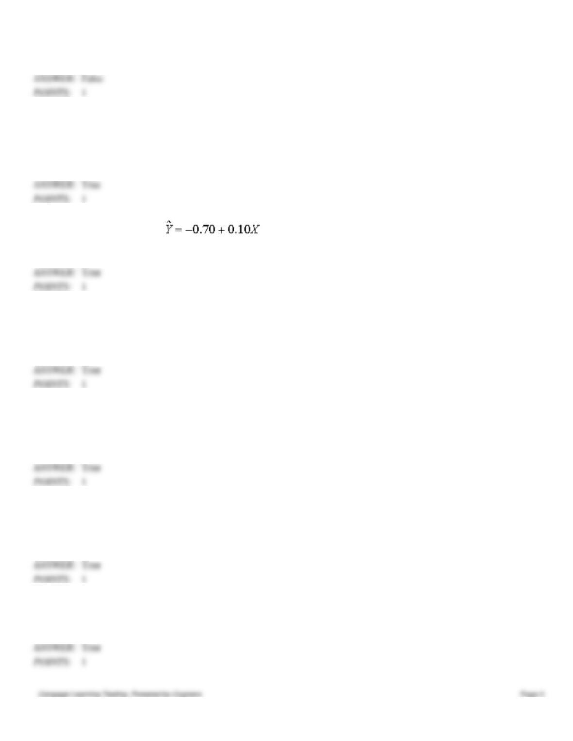
14. In reference to the equation , the value 0.10 is the expected change in Y per unit change in X.
a.
True
b.
False
True
1
15. In regression analysis, we can often use the standard error of estimate se to judge which of several potential regression
equations is the most useful.
a.
True
b.
False
True
1
16. The percentage of variation explained R2 is the square of the correlation between the observed Y values and the fitted
Y values.
a.
True
b.
False
True
1
17. The adjusted R2 is used primarily to monitor whether extra explanatory variables really belong in a multiple regression
model.
a.
True
b.
False
True
1
18. A time series can consist of four different components: trend, seasonal, cyclical, and random (or noise).
a.
True
b.
False
1
19. The smoothing constant used in simple exponential smoothing is analogous to the span in moving averages.
a.
True
b.
False
True
1
20. Winter’s method is an exponential smoothing method, which is appropriate for a series with trend but no seasonality.
a.
True
b.
False
False
1
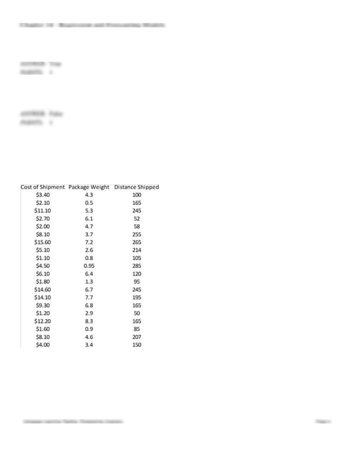
Exhibit 14-1
An express delivery service company recently conducted a study to investigate the relationship between the cost of
shipping a package (Y), the package weight in pounds (X1), and the distance shipped in miles (X2). Twenty packages were
randomly selected from among the large number received for shipment, and a detailed analysis of the shipping cost was
conducted for each package. The sample information is shown in the table below:
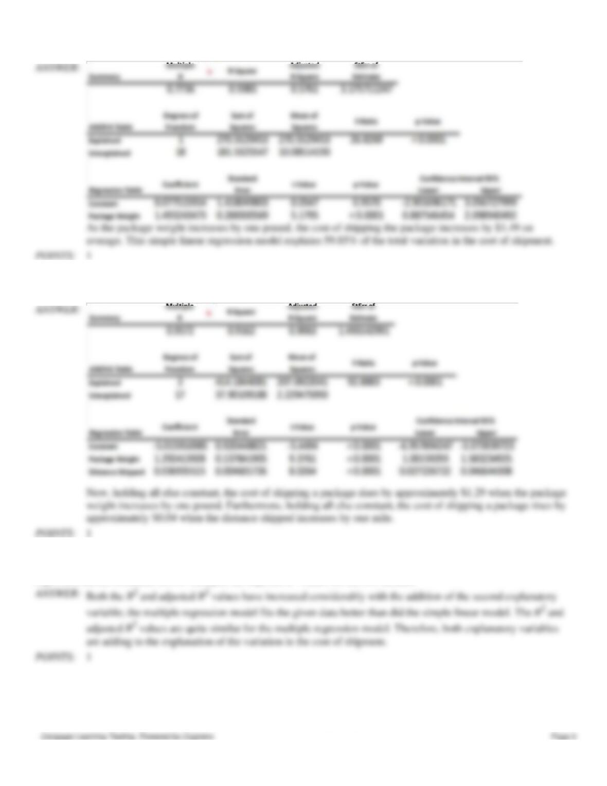
21. Refer to Exhibit 14–1. Estimate a simple linear regression model involving shipping cost and package weight. Interpret
the slope coefficient of the least squares line as well as R2.
Chapter 14 – Regression and Forecasting Models
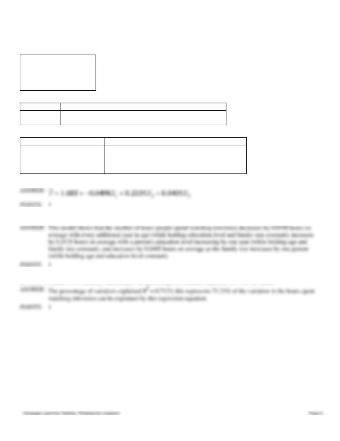
22. Refer to Exhibit 14–1. Add the second explanatory variable (distance shipped) to the regression model. Estimate and
interpret the slopes of this expanded model.
23. Refer to Exhibit 14–1. How does the R2 value for this multiple regression model compare to that of the simple
regression model estimated above? Interpret the adjusted R2 values for the two models.
Exhibit 14-2
The station manager of a local television station is interested in predicting the amount of television (in hours) that people
will watch in the viewing area. The explanatory variables are: X1 age (in years), X2 education (highest level obtained, in
Chapter 14 – Regression and Forecasting Models
years) and X3 family size (number of family members in household). The multiple regression output is shown below:
Summary measures
Multiple R
0.8440
R-Square
0.7123
Adj R-Square
0.6644
StErr of
Estimate
0.5598
ANOVA Table
Source
df
SS
MS
F
p-value
Explained
3
13.9682
4.6561
14.8564
0.0000
Unexplained
18
5.6413
0.3134
Regression coefficients
Coefficient
Std Err
t-value
p-value
Constant
1.683
1.1696
1.4389
0.1674
Age
−0.0498
0.0199
−2.5018
0.0222
Education
0.2135
0.0503
4.2426
0.0005
Family Size
0.0405
0.0784
0.5168
0.6116
24. Refer to Exhibit 14–2. Use the information above to estimate the linear regression model.
POINTS:
1
25. Refer to Exhibit 14–2. Interpret each of the estimated regression coefficients of the regression model above.
family size constant), and increases by 0.0405 hours on average as the family size increases by one person
(while holding age and education level constant).
POINTS:
1
26. Refer to Exhibit 14–2. Identify and interpret the percentage of variation explained (R2) for the model.
watching television can be explained by this regression equation.
POINTS:
1
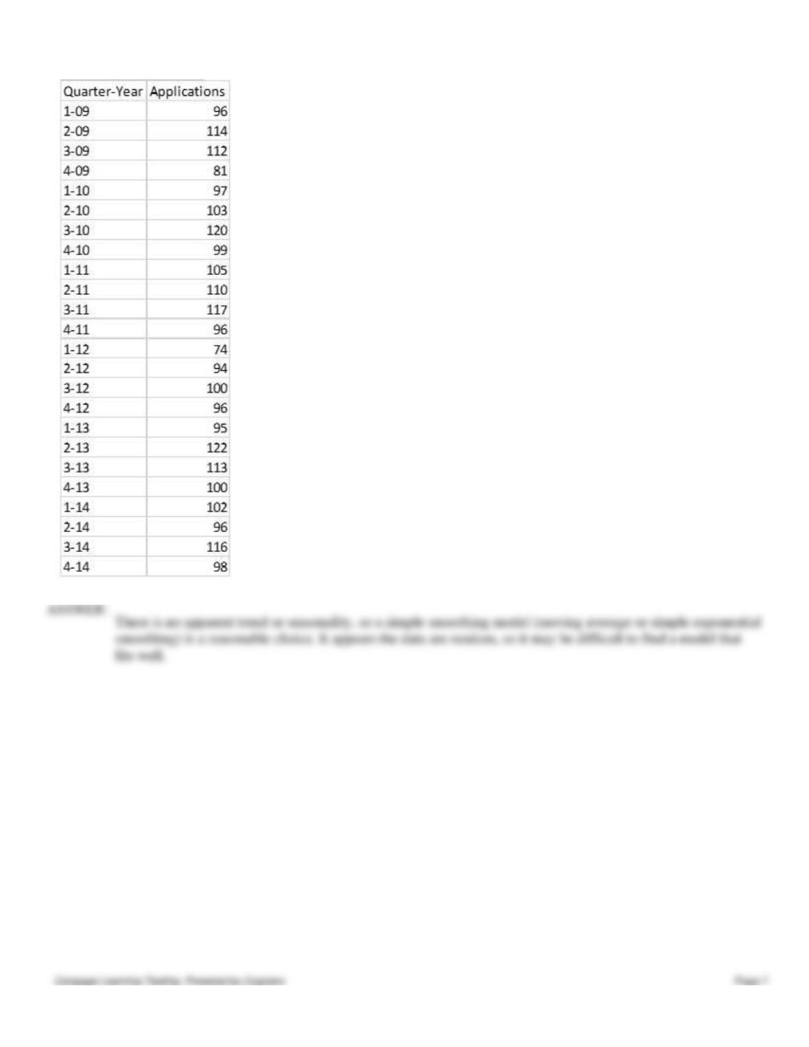
Exhibit 14-3
The quarterly numbers of applications for home mortgage loans at a branch office of a large bank are recorded in the table
below.
27. Refer to Exhibit 14–3. Obtain a time series chart. Which of the forecasting models (one or more) do you think should
be used for forecasting based on this chart? Why?
Chapter 14 – Regression and Forecasting Models
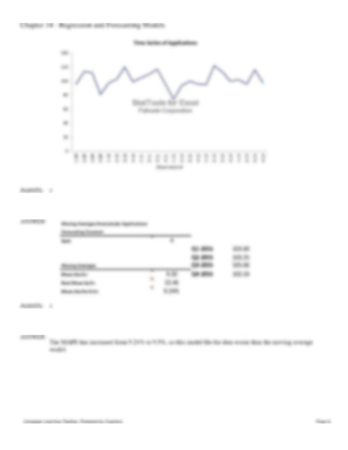
28. Refer to Exhibit 14–3. Use a moving average model to forecast these data, requesting 4 quarters of future forecasts.
Use a span of 4 quarters.
29. Refer to Exhibit 14–3. Use simple exponential smoothing to forecast these data, requesting 4 quarters of future
forecasts. Use the default smoothing constant of 0.10. Is this better than the moving average model?
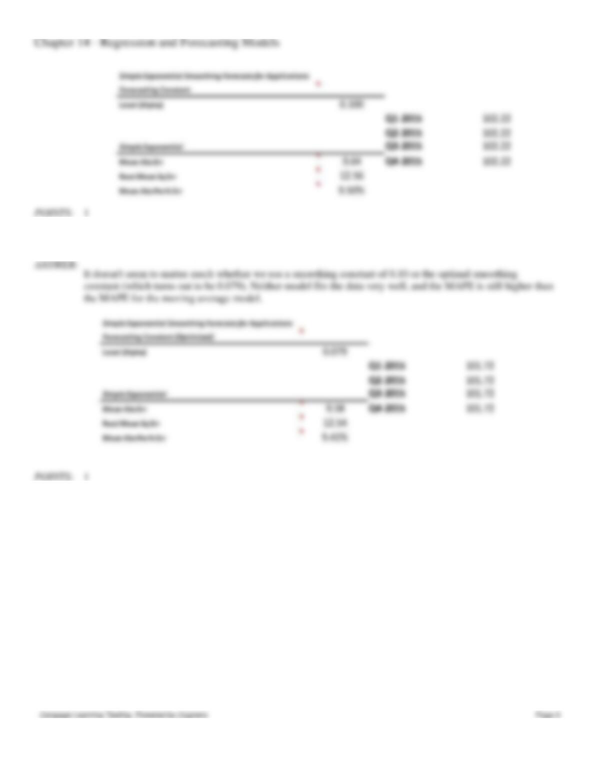
30. Refer to Exhibit 14–3. Obtain a simple exponential smoothing forecast again, this time optimizing the smoothing
constant. Does it make much of an improvement?