Introduction to Multiple Regression 14-1
CHAPTER 14: INTRODUCTION TO MULTIPLE
REGRESSION
1. In a multiple regression problem involving two independent variables, if b1 is computed to be
+2.0, it means that
a) the relationship between X1 and Y is significant.
b) the estimated mean of Y increases by 2 units for each increase of 1 unit of X1, holding X2
constant.
c) the estimated mean of Y increases by 2 units for each increase of 1 unit of X1, without
regard to X2.
d) the estimated mean of Y is 2 when X1 equals zero.
2. The coefficient of multiple determination r2Y.12
a) measures the variation around the predicted regression equation.
b) measures the proportion of variation in Y that is explained by X1 and X2.
c) measures the proportion of variation in Y that is explained by X1 holding X2 constant.
d) will have the same sign as b1.
3. In a multiple regression model, the value of the coefficient of multiple determination
a) has to fall between -1 and +1.
b) has to fall between 0 and +1.
c) has to fall between -1 and 0.
d) can fall between any pair of real numbers.
4. In a multiple regression model, which of the following is correct regarding the value of the
adjusted 2
r?
a) It can be negative.
b) It has to be positive.
c) It has to be larger than the coefficient of multiple determination.
d) It can be larger than 1.
14-2 Introduction to Multiple Regression
SCENARIO 14-1
A manager of a product sales group believes the number of sales made by an employee (Y) depends
on how many years that employee has been with the company (X1) and how he/she scored on a
business aptitude test (X2). A random sample of 8 employees provides the following:
Employee Y X1 X2
1 100 10 7
2 90 3 10
3 80 8 9
4 70 5 4
5 60 5 8
6 50 7 5
7 40 1 4
8 30 1 1
5. Referring to Scenario 14-1, for these data, what is the value for the regression constant, b0?
a) 0.998
b) 3.103
c) 4.698
d) 21.293
6. Referring to Scenario 14-1, for these data, what is the estimated coefficient for the variable
representing years an employee has been with the company, b1?
a) 0.998
b) 3.103
c) 4.698
d) 21.293
7. Referring to Scenario 14-1, for these data, what is the estimated coefficient for the variable
representing scores on the aptitude test, b2?
a) 0.998
b) 3.103
c) 4.698
d) 21.293
Introduction to Multiple Regression 14-3
8. Referring to Scenario 14-1, if an employee who had been with the company 5 years scored a 9 on
the aptitude test, what would his estimated expected sales be?
a) 79.09
b) 60.88
c) 55.62
d) 17.98
SCENARIO 14-2
A professor of industrial relations believes that an individual’s wage rate at a factory (Y) depends on
his performance rating (X1) and the number of economics courses the employee successfully
completed in college (X2). The professor randomly selects 6 workers and collects the following
information:
Employee Y ($) X1 X2
1 10 3 0
2 12 1 5
3 15 8 1
4 17 5 8
5 20 7 12
6 25 10 9
9. Referring to Scenario 14-2, for these data, what is the value for the regression constant, b0?
a) 0.616
b) 1.054
c) 6.932
d) 9.103
10. Referring to Scenario 14-2, for these data, what is the estimated coefficient for performance
rating, b1?
a) 0.616
b) 1.054
c) 6.932
d) 9.103
14-4 Introduction to Multiple Regression
11. Referring to Scenario 14-2, for these data, what is the estimated coefficient for the number of
economics courses taken, b2?
a) 0.616
b) 1.054
c) 6.932
d) 9.103
12. Referring to Scenario 14-2, suppose an employee had never taken an economics course and
managed to score a 5 on his performance rating. What is his estimated expected wage rate?
a) 10.90
b) 12.20
c) 17.23
d) 25.11
13. Referring to Scenario 14-2, an employee who took 12 economics courses scores 10 on the
performance rating. What is her estimated expected wage rate?
a) 10.90
b) 12.20
c) 24.87
d) 25.70
14. The variation attributable to factors other than the relationship between the independent variables
and the explained variable in a regression analysis is represented by
a) regression sum of squares.
b) error sum of squares.
c) total sum of squares.
d) regression mean squares.

Introduction to Multiple Regression 14-5
SCENARIO 14-3
An economist is interested to see how consumption for an economy (in $ billions) is influenced by
gross domestic product ($ billions) and aggregate price (consumer price index). The Microsoft Excel
output of this regression is partially reproduced below.
SUMMARY OUTPUT
Regression Statistics
Multiple R 0.991
R Square 0.982
Adjusted R Square 0.976
Standard Error 0.299
Observations 10
ANOVA
df SS MS F Signif F
Regression 2 33.4163 16.7082 186.325 0.0001
Residual 7 0.6277 0.0897
Total 9 34.0440
Coeff StdError t Stat P-value
Intercept – 0.0861 0.5674 – 0.152 0.8837
GDP 0.7654 0.0574 13.340 0.0001
Price – 0.0006 0.0028 – 0.219 0.8330
15. Referring to Scenario 14-3, when the economist used a simple linear regression model with
consumption as the dependent variable and GDP as the independent variable, he obtained an r2
value of 0.971. What additional percentage of the total variation of consumption has been
explained by including aggregate prices in the multiple regression?
a) 98.2
b) 11.1
c) 2.8
d) 1.1
16. Referring to Scenario 14-3, the p-value for GDP is
a) 0.05
b) 0.01
c) 0.001
d) None of the above.
14-6 Introduction to Multiple Regression
17. Referring to Scenario 14-3, the p-value for the aggregated price index is
a) 0.05
b) 0.01
c) 0.001
d) None of the above.
18. Referring to Scenario 14-3, the p-value for the regression model as a whole is
a) 0.05
b) 0.01
c) 0.001
d) None of the above.
19. Referring to Scenario 14-3, what is the predicted consumption level for an economy with GDP
equal to $4 billion and an aggregate price index of 150?
a) $1.39 billion
b) $2.89 billion
c) $4.75 billion
d) $9.45 billion
20. Referring to Scenario 14-3, what is the estimated mean consumption level for an economy with
GDP equal to $4 billion and an aggregate price index of 150?
a) $1.39 billion
b) $2.89 billion
c) $4.75 billion
d) $9.45 billion
Introduction to Multiple Regression 14-7
21. Referring to Scenario 14-3, what is the estimated mean consumption level for an economy with
GDP equal to $2 billion and an aggregate price index of 90?
a) $1.39 billion
b) $2.89 billion
c) $4.75 billion
d) $9.45 billion
22. Referring to Scenario 14-3, one economy in the sample had an aggregate consumption level of $3
billion, a GDP of $3.5 billion, and an aggregate price level of 125. What is the residual for this
data point?
a) $2.52 billion
b) $0.48 billion
c) – $1.33 billion
d) – $2.52 billion
23. Referring to Scenario 14-3, one economy in the sample had an aggregate consumption level of $4
billion, a GDP of $6 billion, and an aggregate price level of 200. What is the residual for this data
point?
a) $4.39 billion
b) $0.39 billion
c) – $0.39 billion
d) – $1.33 billion
24. Referring to Scenario 14-3, to test for the significance of the coefficient on aggregate price index,
the value of the relevant t-statistic is
a) 2.365
b) 0.143
c) – 0.219
d) – 1.960
14-8 Introduction to Multiple Regression
25. Referring to Scenario 14-3, to test for the significance of the coefficient on aggregate price index,
the p-value is
a) 0.0001
b) 0.8330
c) 0.8837
d) 0.9999
26. Referring to Scenario 14-3, to test for the significance of the coefficient on gross domestic
product, the p-value is
a) 0.0001
b) 0.8330
c) 0.8837
d) 0.9999
27. Referring to Scenario 14-3, to test whether aggregate price index has a negative impact on
consumption, the p-value is _______?
a) 0.0001
b) 0.4165
c) 0.8330
d) 0.8837
28. Referring to Scenario 14-3, to test whether aggregate price index has a positive impact on
consumption, the p-value is
a) 0.0001
b) 0.4165
c) 0.5835
d) 0.8330

Introduction to Multiple Regression 14-9
29. Referring to Scenario 14-3, to test whether gross domestic product has a positive impact on
consumption, the p-value is
a) 0.00005
b) 0.0001
c) 0.9999
d) 0.99995
SCENARIO 14-4
A real estate builder wishes to determine how house size (House) is influenced by family income
(Income) and family size (Size). House size is measured in hundreds of square feet and income is
measured in thousands of dollars. The builder randomly selected 50 families and ran the multiple
regression. Partial Microsoft Excel output is provided below:
Regression Statistics
Multiple R 0.8479
R Square 0.7189
Adjusted R Square 0.7069
Standard Error 17.5571
Observations 50
ANOVA
df SS MS F Significance F
Regression 37043.3236 18521.6618 0.0000
Residual 14487.7627 308.2503
Total 49 51531.0863
Coefficients Standard Error t Stat P-value
Intercept -5.5146 7.2273 -0.7630 0.4493
Income 0.4262 0.0392 10.8668 0.0000
Size 5.5437 1.6949 3.2708 0.0020
Also
()
12
|SSR X X =36400.6326 and
()
21
| 3297.7917SSR X X =
14-10 Introduction to Multiple Regression
30. Referring to Scenario 14-4, what fraction of the variability in house size is explained by income
and size of family?
a) 17.56%
b) 70.69%
c) 71.89%
d) 84.79%
31. Referring to Scenario 14-4, which of the independent variables in the model are significant at the
5% level?
a) Income only
b) Size only
c) Income and Size
d) None
32. Referring to Scenario 14-4, when the builder used a simple linear regression model with house
size (House) as the dependent variable and family size (Size) as the independent variable, he
obtained an r2 value of 1.25%. What additional percentage of the total variation in house size has
been explained by including income in the multiple regression?
a) 15.00%
b) 70.64%
c) 71.50%
d) 73.62%
33. Referring to Scenario 14-4, which of the following values for the level of significance is the
smallest for which each explanatory variable is significant individually?
a) 0.001
b) 0.010
c) 0.025
d) 0.050
Introduction to Multiple Regression 14-11
34. Referring to Scenario 14-4, which of the following values for the level of significance is the
smallest for which at least one explanatory variable is significant individually?
a) 0.005
b) 0.010
c) 0.025
d) 0.050
35. Referring to Scenario 14-4, which of the following values for the level of significance is the
smallest for which at most one explanatory variable is significant individually?
a) 0.001
b) 0.010
c) 0.025
d) 0.050
36. Referring to Scenario 14-4, which of the following values for the level of significance is the
smallest for which the regression model as a whole is significant?
a) 0.0005
b) 0.001
c) 0.01
d) 0.05
37. Referring to Scenario 14-4, what is the predicted house size (in hundreds of square feet) for an
individual earning an annual income of $40,000 and having a family size of 4?
38. Referring to Scenario 14-4, what annual income (in thousands of dollars) would an individual
with a family size of 4 need to attain a predicted 10,000 square foot home (House = 100)?
14-12 Introduction to Multiple Regression
39. Referring to Scenario 14-4, what annual income (in thousands of dollars) would an individual
with a family size of 9 need to attain a predicted 5,000 square foot home (House = 50)?
40. Referring to Scenario 14-4, one individual in the sample had an annual income of $100,000 and a
family size of 10. This individual owned a home with an area of 7,000 square feet (House =
70.00). What is the residual (in hundreds of square feet) for this data point?
41. Referring to Scenario 14-4, one individual in the sample had an annual income of $40,000 and a
family size of 1. This individual owned a home with an area of 1,000 square feet (House =
10.00). What is the residual (in hundreds of square feet) for this data point?
42. Referring to Scenario 14-4, suppose the builder wants to test whether the coefficient on Income is
significantly different from 0. What is the value of the relevant t-statistic?
a) -0.7630
b) 3.2708
c) 10.8668
d) 60.0864
Introduction to Multiple Regression 14-13
43. Referring to Scenario 14-4, at the 0.01 level of significance, what conclusion should the builder
reach regarding the inclusion of Income in the regression model?
a) Income is significant in explaining house size and should be included in the model
because its p-value is less than 0.01.
b) Income is significant in explaining house size and should be included in the model
because its p-value is more than 0.01.
c) Income is not significant in explaining house size and should not be included in the
model because its p-value is less than 0.01.
d) Income is not significant in explaining house size and should not be included in the
model because its p-value is more than 0.01.
44. Referring to Scenario 14-4, suppose the builder wants to test whether the coefficient on Size is
significantly different from 0. What is the value of the relevant t-statistic?
a) -0.7630
b) 3.2708
c) 10.8668
d) 60.0864
45. Referring to Scenario 14-4, at the 0.01 level of significance, what conclusion should the builder
draw regarding the inclusion of Size in the regression model?
a) Size is significant in explaining house size and should be included in the model because
its p-value is less than 0.01.
b) Size is significant in explaining house size and should be included in the model because
its p-value is more than 0.01.
c) Size is not significant in explaining house size and should not be included in the model
because its p-value is less than 0.01.
d) Size is not significant in explaining house size and should not be included in the model
because its p-value is more than 0.01.
46. Referring to Scenario 14-4, what is the value of the calculated F test statistic that is missing from
the output for testing whether the whole regression model is significant?
14-14 Introduction to Multiple Regression
47. Referring to Scenario 14-4, the observed value of the F-statistic is missing from the printout.
What are the degrees of freedom for this F-statistic?
a) 2 for the numerator, 47 for the denominator
b) 2 for the numerator, 49 for the denominator
c) 49 for the numerator, 47 for the denominator
d) 47 for the numerator, 49 for the denominator
48. Referring to Scenario 14-4, what are the regression degrees of freedom that are missing from the
output?
a) 2
b) 47
c) 49
d) 50
49. Referring to Scenario 14-4, what are the residual degrees of freedom that are missing from the
output?
a) 2
b) 47
c) 49
d) 50
50. Referring to Scenario 14-4 and allowing for a 1% probability of committing a type I error, what is
the decision and conclusion for the test 01 2 1
: 0 vs. : At least one 0, 1, 2
j
HH j
ββ β
== ≠ = ?
a) Do not reject H0 and conclude that the 2 independent variables taken as a group have
significant linear effects on house size.
b) Do not reject H0 and conclude that the 2 independent variables taken as a group do not
have significant linear effects on house size.
c) Reject H0 and conclude that the 2 independent variables taken as a group have significant
linear effects on house size.
d) Reject H0 and conclude that the 2 independent variables taken as a group do not have
significant linear effects on house size.
Introduction to Multiple Regression 14-15
51. Referring to Scenario 14-4, the value of the partial F test statistic is ____ for
H0 : Variable X1 does not significantly improve the model after variable X2 has been included
H1 : Variable X1 significantly improves the model after variable X2 has been included
52. Referring to Scenario 14-4, the partial F test for
H0 : Variable X1 does not significantly improve the model after variable X2 has been included
H1 : Variable X1 significantly improves the model after variable X2 has been included
has ____ and ____ degrees of freedom.
53. Referring to Scenario 14-4, the value of the partial F test statistic is ____ for
H0 : Variable X2 does not significantly improve the model after variable X1 has been included
H1 : Variable X2 significantly improves the model after variable X1 has been included
54. Referring to Scenario 14-4, the partial F test for
H0 : Variable X2 does not significantly improve the model after variable X1 has been included
H1 : Variable X2 significantly improves the model after variable X1 has been included
has ____ and ____ degrees of freedom.
55. Referring to Scenario 14-4, the coefficient of partial determination 2
12Y
r⋅ is ____.
56. Referring to Scenario 14-4, the coefficient of partial determination 2
21Y
r⋅ is ____.
57. Referring to Scenario 14-4, ____% of the variation in the house size can be explained by the
variation in the family income while holding the family size constant.
58. Referring to Scenario 14-4, ____% of the variation in the house size can be explained by the
variation in the family size while holding the family income constant.
SCENARIO 14-5
A microeconomist wants to determine how corporate sales are influenced by capital and wage
spending by companies. She proceeds to randomly select 26 large corporations and record
information in millions of dollars. The Microsoft Excel output below shows results of this multiple
regression.
SUMMARY OUTPUT
Regression Statistics
Multiple R 0.830
R Square 0.689
Adjusted R Square 0.662
Standard Error 17501.643
Observations 26
ANOVA
df SS MS F Signif F
Regression 2 15579777040 7789888520 25.432 0.0001
Residual 23 7045072780 306307512
Total 25 22624849820
Coeff StdError t Stat P-value
Intercept 15800.0000 6038.2999 2.617 0.0154
Capital 0.1245 0.2045 0.609 0.5485
Wages 7.0762 1.4729 4.804 0.0001
Introduction to Multiple Regression 14-17
59. Referring to Scenario 14-5, what fraction of the variability in sales is explained by spending on
capital and wages?
a) 27.0%
b) 50.9%
c) 68.9%
d) 83.0%
60. Referring to Scenario 14-5, which of the independent variables in the model are significant at the
5% level?
a) Capital, Wages
b) Capital
c) Wages
d) None of the above
61. Referring to Scenario 14-5, when the microeconomist used a simple linear regression model with
sales as the dependent variable and wages as the independent variable, she obtained an r2 value of
0.601. What additional percentage of the total variation of sales has been explained by including
capital spending in the multiple regression?
a) 60.1%
b) 31.1%
c) 22.9%
d) 8.8%
62. Referring to Scenario 14-5, what is the p-value for Wages?
a) 0.01
b) 0.05
c) 0.0001
d) None of the above
14-18 Introduction to Multiple Regression
63. Referring to Scenario 14-5, what is the p-value for testing whether Wages have a positive impact
on corporate sales?
a) 0.01
b) 0.05
c) 0.0001
d) 0.00005
64. Referring to Scenario 14-5, what is the p-value for testing whether Wages have a negative impact
on corporate sales?
a) 0.05
b) 0.0001
c) 0.00005
d) 0.99995
65. Referring to Scenario 14-5, what is the p-value for Capital?
a) 0.01
b) 0.025
c) 0.05
d) None of the above
66. Referring to Scenario 14-5, what is the p-value for testing whether Capital has a positive
influence on corporate sales?
a) 0.025
b) 0.05
c) 0.2743
d) 0.5485
Introduction to Multiple Regression 14-19
67. Referring to Scenario 14-5, what is the p-value for testing whether Capital has a negative
influence on corporate sales?
a) 0.05
b) 0.2743
c) 0.5485
d) 0.7258
68. Referring to Scenario 14-5, which of the following values for
α
is the smallest for which the
regression model as a whole is significant?
a) 0.00005
b) 0.001
c) 0.01
d) 0.05
69. Referring to Scenario 14-5, what are the predicted sales (in millions of dollars) for a company
spending $100 million on capital and $100 million on wages?
a) 15,800.00
b) 16,520.07
c) 17,277.49
d) 20,455.98
70. Referring to Scenario 14-5, what are the predicted sales (in millions of dollars) for a company
spending $500 million on capital and $200 million on wages?
a) 15,800.00
b) 16,520.07
c) 17,277.49
d) 20,455.98
14-20 Introduction to Multiple Regression
71. Referring to Scenario 14-5, one company in the sample had sales of $20 billion (Sales = 20,000).
This company spent $300 million on capital and $700 million on wages. What is the residual (in
millions of dollars) for this data point?
a) 874.55
b) 622.87
c) –790.69
d) –983.56
72. Referring to Scenario 14-5, one company in the sample had sales of $21.439 billion (Sales =
21,439). This company spent $300 million on capital and $700 million on wages. What is the
residual (in millions of dollars) for this data point?
a) 790.69
b) 648.31
c) –648.31
d) –790.69
73. Referring to Scenario 14-5, suppose the microeconomist wants to test whether the coefficient on
Capital is significantly different from 0. What is the value of the relevant t-statistic?
a) 0.609
b) 2.617
c) 4.804
d) 25.432
Introduction to Multiple Regression 14-21
74. Referring to Scenario 14-5, at the 0.01 level of significance, what conclusion should the
microeconomist reach regarding the inclusion of Capital in the regression model?
a) Capital is significant in explaining corporate sales and should be included in the model
because its p-value is less than 0.01.
b) Capital is significant in explaining corporate sales and should be included in the model
because its p-value is more than 0.01.
c) Capital is not significant in explaining corporate sales and should not be included in the
model because its p-value is less than 0.01.
d) Capital is not significant in explaining corporate sales and should not be included in the
model because its p-value is more than 0.01.
75. Referring to Scenario 14-5, the observed value of the F-statistic is given on the printout as
25.432. What are the degrees of freedom for this F-statistic?
a) 25 for the numerator, 2 for the denominator
b) 2 for the numerator, 23 for the denominator
c) 23 for the numerator, 25 for the denominator
d) 2 for the numerator, 25 for the denominator

14-22 Introduction to Multiple Regression
SCENARIO 14-6
One of the most common questions of prospective house buyers pertains to the cost of heating in
dollars (Y). To provide its customers with information on that matter, a large real estate firm used the
following 2 variables to predict heating costs: the daily minimum outside temperature in degrees of
Fahrenheit ( 1
X
) and the amount of insulation in inches ( 2
X
). Given below is EXCEL output of the
regression model.
Regression Statistics
Multiple R 0.5270
R Square 0.2778
Adjusted R Square 0.1928
Standard Error 40.9107
Observations 20
ANOVA
df SS MS F Significance F
Regression 2 10943.0190 5471.5095 3.2691 0.0629
Residual 17 28452.6027 1673.6825
Total 19 39395.6218
Coefficients Standard Error t Stat P-value Lower 95% Upper 95%
Intercept 448.2925 90.7853 4.9379 0.0001 256.7522 639.8328
Temperature -2.7621 1.2371 -2.2327 0.0393 -5.3721 -0.1520
Insulation -15.9408 10.0638 -1.5840 0.1316 -37.1736 5.2919
Also
()
12
|SSR X X =8343.3572 and
()
21
|SSR X X =4199.2672
76. Referring to Scenario 14-6, the estimated value of the regression parameter 1
β
in means that
a) holding the effect of the amount of insulation constant, an estimated expected $1 increase
in heating costs is associated with a decrease in the daily minimum outside temperature
by 2.76 degrees.
b) holding the effect of the amount of insulation constant, a 1 degree increase in the daily
minimum outside temperature results in a decrease in heating costs by $2.76.
c) holding the effect of the amount of insulation constant, a 1 degree increase in the daily
minimum outside temperature results in an estimated decrease in mean heating costs by
$2.76.
d) holding the effect of the amount of insulation constant, a 1% increase in the daily
minimum outside temperature results in an estimated decrease in mean heating costs by
2.76%.
Introduction to Multiple Regression 14-23
77. Referring to Scenario 14-6, what can we say about the regression model?
a) The model explains 17.12% of the variability of heating costs; after correcting for the
degrees of freedom, the model explains 27.78% of the sample variability of heating costs.
b) The model explains 19.28% of the variability of heating costs; after correcting for the
degrees of freedom, the model explains 27.78% of the sample variability of heating costs.
c) The model explains 27.78% of the variability of heating costs; after correcting for the
degrees of freedom, the model explains 19.28% of the sample variability of heating costs.
d) The model explains 19.28% of the variability of heating costs; after correcting for the
degrees of freedom, the model explains 17.12% of the sample variability of heating costs.
78. Referring to Scenario 14-6, what is your decision and conclusion for the test
02 12
: 0 vs. : 0HH
ββ
=≠
at the
α
= 0.01 level of significance?
a) Do not reject H0 and conclude that the amount of insulation has a linear effect on heating
costs.
b) Reject H0 and conclude that the amount of insulation does not have a linear effect on
heating costs.
c) Reject H0 and conclude that the amount of insulation has a linear effect on heating costs.
d) Do not reject H0 and conclude that the amount of insulation does not have a linear effect
on heating costs.
79. Referring to Scenario 14-6, what is the 95% confidence interval for the expected change in
heating costs as a result of a 1 degree Fahrenheit change in the daily minimum outside
temperature?
a) [256.7522, 639.8328]
b) [204.7854, 497.1733]
c) [−5.3721, −0.1520]
d) [−37.1736, 5.2919]
14-24 Introduction to Multiple Regression
80. Referring to Scenario 14-6 and allowing for a 1% probability of committing a type I error, what is
the decision and conclusion for the test 01 2 1
: 0 vs. : At least one 0, 1, 2
j
HH j
ββ β
== ≠ = ?
a) Do not reject H0 and conclude that the 2 independent variables taken as a group have
significant linear effects on heating costs.
b) Do not reject H0 and conclude that the 2 independent variables taken as a group do not
have significant linear effects on heating costs.
c) Reject H0 and conclude that the 2 independent variables taken as a group have significant
linear effects on heating costs.
d) Reject H0 and conclude that the 2 independent variables taken as a group do not have
significant linear effects on heating costs.
81. Referring to Scenario 14-6, the value of the partial F test statistic is ____ for
H0 : Variable X1 does not significantly improve the model after variable X2 has been included
H1 : Variable X1 significantly improves the model after variable X2 has been included
82. Referring to Scenario 14-6, the partial F test for
H0 : Variable X1 does not significantly improve the model after variable X2 has been included
H1 : Variable X1 significantly improves the model after variable X2 has been included
has ____ and ____ degrees of freedom.
83. Referring to Scenario 14-6, the value of the partial F test statistic is ____ for
H0 : Variable X2 does not significantly improve the model after variable X1 has been included
H1 : Variable X2 significantly improves the model after variable X1 has been included
Introduction to Multiple Regression 14-25
84. Referring to Scenario 14-6, the partial F test for
H0 : Variable X2 does not significantly improve the model after variable X1 has been included
H1 : Variable X2 significantly improves the model after variable X1 has been included
has ____ and ____ degrees of freedom.
85. Referring to Scenario 14-6, the coefficient of partial determination 2
12Y
r⋅ is ____.
86. Referring to Scenario 14-6, the coefficient of partial determination 2
21Y
r⋅ is ____.
87. Referring to Scenario 14-6, ____% of the variation in heating cost can be explained by the
variation in minimum outside temperature while holding the amount of insulation constant.
88. Referring to Scenario 14-6, ____% of the variation in heating cost can be explained by the
variation in the amount of insulation while holding the minimum outside temperature constant.
89. True or False: The interpretation of the slope is different in a multiple linear regression model as
compared to a simple linear regression model.
14-26 Introduction to Multiple Regression
90. True or False: The coefficient of multiple determination r2Y.12 measures the proportion of
variation in Y that is explained by X1 and X2.
91. True or False: When an additional explanatory variable is introduced into a multiple regression
model, the coefficient of multiple determination will never decrease.
92. True or False: When an additional explanatory variable is introduced into a multiple regression
model, the adjusted 2
rcan never decrease.
93. True or False: When an explanatory variable is dropped from a multiple regression model, the
coefficient of multiple determination can increase.
94. True or False: When an explanatory variable is dropped from a multiple regression model, the
adjusted 2
rcan increase.
95. True or False: The slopes in a multiple regression model are called net regression coefficients.
Introduction to Multiple Regression 14-27
96. True or False: In calculating the standard error of the estimate, SYX =MSE , there are n – k – 1
degrees of freedom, where n is the sample size and k represents the number of independent
variables in the model.
97. True or False: The total sum of squares (SST) in a regression model will never be greater than the
regression sum of squares (SSR).
98. True or False: The coefficient of multiple determination measures the proportion of the total
variation in the dependent variable that is explained by the set of independent variables.
99. True or False: The coefficient of multiple determination is calculated by taking the ratio of the
regression sum of squares over the total sum of squares (SSR/SST) and subtracting that value from
1.
100. True or False: In a particular model, the sum of the squared residuals was 847. If the model
had 5 independent variables, and the data set contained 40 points, the value of the standard error
of the estimate is 24.911.
101. True or False: A multiple regression is called “multiple” because it has several data points.
14-28 Introduction to Multiple Regression
102. True or False: A multiple regression is called “multiple” because it has several explanatory
variables.
103. True or False: If you have taken into account all relevant explanatory factors, the residuals
from a multiple regression model should be random.
104. True or False: Multiple regression is the process of using several independent variables to
predict a number of dependent variables.
105. True or False: You have just computed a regression model in which the value of coefficient of
multiple determination is 0.57. To determine if this indicates that the independent variables
explain a significant portion of the variation in the dependent variable, you would perform an F–
test.
106. True or False: From the coefficient of multiple determination, you cannot detect the strength
of the relationship between Y and any individual independent variable.
107. True or False: Consider a regression in which b2 = – 1.5 and the standard error of this
coefficient equals 0.3. To determine whether X2 is a significant explanatory variable, you would
compute an observed t-value of – 5.0.
Introduction to Multiple Regression 14-29
108. True or False: A regression had the following results: SST = 82.55, SSE = 29.85. It can be said
that 73.4% of the variation in the dependent variable is explained by the independent variables in
the regression.
109. True or False: A regression had the following results: SST = 82.55, SSE = 29.85. It can be said
that 63.84% of the variation in the dependent variable is explained by the independent variables
in the regression.
110. True or False: A regression had the following results: SST = 102.55, SSE = 82.04. It can be
said that 90.0% of the variation in the dependent variable is explained by the independent
variables in the regression.
111. True or False: A regression had the following results: SST = 102.55, SSE = 82.04. It can be
said that 20.0% of the variation in the dependent variable is explained by the independent
variables in the regression.
14-30 Introduction to Multiple Regression
SCENARIO 14-7
The department head of the accounting department wanted to see if she could predict the GPA of
students using the number of course units (credits) and total SAT scores of each. She takes a sample
of students and generates the following Microsoft Excel output:
SUMMARY OUTPUT
Regression Statistics
Multiple R 0.916
R Square 0.839
Adjusted R Square 0.732
Standard Error 0.24685
Observations 6
ANOVA
df SS MS F Signif F
Regression 2 0.95219 0.47610 7.813 0.0646
Residual 3 0.18281 0.06094
Total 5 1.13500
Coeff StdError t Stat P-value
Intercept 4.593897 1.13374542 4.052 0.0271
Units – 0.247270 0. 06268485 – 3.945 0.0290
SAT Total 0.001443 0.00101241 1.425 0.2494
112. Referring to Scenario 14-7, the estimate of the unit change in the mean of Y per unit change in
X1, holding X2 constant, is ________.
113. Referring to Scenario 14-7, the net regression coefficient of X2 is ________.
114. Referring to Scenario 14-7, the predicted GPA for a student carrying 15 course units and who
has a total SAT of 1,100 is ________.
Introduction to Multiple Regression 14-31
115. Referring to Scenario 14-7, the value of the coefficient of multiple determination, r2Y.12, is
________.
116. Referring to Scenario 14-7, the value of the adjusted coefficient of multiple determination, r2adj,
is ________.
117. Referring to Scenario 14-7, the department head wants to test H0:
β
1=
β
2=0. The appropriate
alternative hypothesis is ________.
118. Referring to Scenario 14-7, the department head wants to test H0:
β
1=
β
2=0. The critical
value of the F test for a level of significance of 0.05 is ________.
119. Referring to Scenario 14-7, the department head wants to test H0:
β
1=
β
2=0. The value of
the F-test statistic is ________.
120. Referring to Scenario 14-7, the department head wants to test H0:
β
1=
β
2=0. The p-value of
the test is ________.
14-32 Introduction to Multiple Regression
121. True or False: Referring to Scenario 14-7, the department head wants to test H0:
β
1=
β
2=0.
At a level of significance of 0.05, the null hypothesis is rejected.
122. Referring to Scenario 14-7, the department head wants to use a t test to test for the significance
of the coefficient of X1. For a level of significance of 0.05, the critical values of the test are
________.
123. Referring to Scenario 14-7, the department head wants to use a t test to test for the significance
of the coefficient of X1. The value of the test statistic is ________.
124. Referring to Scenario 14-7, the department head wants to use a t test to test for the
significance of the coefficient of X1. The p-value of the test is ________.
125. True or False: Referring to Scenario 14-7, the department head wants to use a t test to test for
the significance of the coefficient of X1. At a level of significance of 0.05, the department head
would decide that
β
1≠0.
126. Referring to Scenario 14-7, the department head decided to construct a 95% confidence interval
for
β
1. The confidence interval is from ________ to ________.

Introduction to Multiple Regression 14-33
SCENARIO 14-8
A financial analyst wanted to examine the relationship between salary (in $1,000) and 2 variables:
age (X1 = Age) and experience in the field (X2 = Exper). He took a sample of 20 employees and
obtained the following Microsoft Excel output:
Regression Statistics
Multiple R 0.8535
R Square 0.7284
Adjusted R Square 0.6964
Standard Error 10.5630
Observations 20
ANOVA
df SS MS F Significance F
Regression 2 5086.5764 2543.2882 22.7941 0.0000
Residual 17 1896.8050 111.5768
Total 19 6983.3814
Coefficients Standard Error t Stat P-value Lower 95%
Upper
95%
Intercept 1.5740 9.2723 0.1698 0.8672 -17.9888 21.1368
Age 1.3045 0.1956 6.6678 0.0000 0.8917 1.7173
Exper -0.1478 0.1944 -0.7604 0.4574 -0.5580 0.2624
Also the sum of squares due to the regression for the model that includes only Age is 5022.0654 while the
sum of squares due to the regression for the model that includes only Exper is 125.9848.
127. Referring to Scenario 14-8, the estimate of the unit change in the mean of Y per unit change in
X1, taking into account the effects of the other variable, is ________.
128. Referring to Scenario 14-8, the estimated change in the mean salary (in $1,000) when an
employee is a year older holding experience constant is ________.
14-34 Introduction to Multiple Regression
129. Referring to Scenario 14-8, the estimated change in the mean salary (in $1,000) for an
employee who has one additional year of experience holding age constant is ________.
130. Referring to Scenario 14-8, the predicted salary (in $1,000) for a 35-year-old person with 10
years of experience is ________.
131. Referring to Scenario 14-8, the value of the coefficient of multiple determination is ________.
132. Referring to Scenario 14-8, the value of the adjusted coefficient of multiple determination is
________.
133. Referring to Scenario 14-8, the analyst wants to use an F-test to test 01 2
: 0H
ββ
==
. The
appropriate alternative hypothesis is ________.
134. Referring to Scenario 14-8, the critical value of an F test on the entire regression for a level of
significance of 0.01 is ________.
Introduction to Multiple Regression 14-35
135. Referring to Scenario 14-8, the value of the F-statistic for testing the significance of the entire
regression is ________.
136. Referring to Scenario 14-8, the p-value of the F test for the significance of the entire regression
is ________.
137. True or False: Referring to Scenario 14-8, the F test for the significance of the entire regression
performed at a level of significance of 0.01 leads to a rejection of the null hypothesis.
138. Referring to Scenario 14-8, the analyst wants to use a t test to test for the significance of the
coefficient of X2. For a level of significance of 0.01, the critical values of the test are ________.
139. Referring to Scenario 14-8, the analyst wants to use a t test to test for the significance of the
coefficient of X2. The value of the test statistic is ________.
140. Referring to Scenario 14-8, the analyst wants to use a t test to test for the significance of the
coefficient of X2. The p-value of the test is ________.
14-36 Introduction to Multiple Regression
141. True or False: Referring to Scenario 14-8, the analyst wants to use a t test to test for the
significance of the coefficient of X2. At a level of significance of 0.01, the department head would
decide that 20
β
≠.
142. Referring to Scenario 14-8, the analyst decided to construct a 95% confidence interval for 2
β
.
The confidence interval is from ________ to ________.
143. Referring to Scenario 14-8, the value of the partial F test statistic is ____ for
H0 : Variable X1 does not significantly improve the model after variable X2 has been included
H1 : Variable X1 significantly improves the model after variable X2 has been included
144. Referring to Scenario 14-8, the partial F test for
H0 : Variable X1 does not significantly improve the model after variable X2 has been included
H1 : Variable X1 significantly improves the model after variable X2 has been included
has ____ and ____ degrees of freedom.
145. Referring to Scenario 14-8, the value of the partial F test statistic is ____ for
H0 : Variable X2 does not significantly improve the model after variable X1 has been included
H1 : Variable X2 significantly improves the model after variable X1 has been included
Introduction to Multiple Regression 14-37
146. Referring to Scenario 14-8, the partial F test for
H0 : Variable X2 does not significantly improve the model after variable X1 has been included
H1 : Variable X2 significantly improves the model after variable X1 has been included
has ____ and ____ degrees of freedom.
147. Referring to Scenario 14-8, the coefficient of partial determination 2
12Y
r⋅ is ____.
148. Referring to Scenario 14-8, the coefficient of partial determination 2
21
Y
r⋅ is ____.
149. Referring to Scenario 14-8, ____% of the variation in salary can be explained by the variation
in age while holding experience constant.
150. Referring to Scenario 14-8, ____% of the variation in salary can be explained by the variation
in experience while holding age constant.
14-38 Introduction to Multiple Regression
SCENARIO 14-9
You decide to predict gasoline prices in different cities and towns in the United States for your term
project. Your dependent variable is price of gasoline per gallon and your explanatory variables are
per capita income and the number of firms that manufacture automobile parts in and around the city.
You collected data of 32 cities and obtained a regression sum of squares SSR= 122.8821. Your
computed value of standard error of the estimate is 1.9549.
151. Referring to Scenario 14-9, what is the value of the coefficient of multiple determination?
152. Referring to Scenario 14-9, the value of adjusted 2
r is
153. Referring to Scenario 14-9, if the variable that measures the number of firms that manufacture
automobile parts in and around the city is removed from the multiple regression model, which of
the following would be true?
a) The adjusted 2
r will definitely increase.
b) The adjusted 2
r cannot increase.
c) The coefficient of multiple determination will not increase.
d) The coefficient of multiple determination will definitely increase.
Introduction to Multiple Regression 14-39
SCENARIO 14-10
You worked as an intern at We Always Win Car Insurance Company last summer. You notice that
individual car insurance premiums depend very much on the age of the individual and the number of
traffic tickets received by the individual. You performed a regression analysis in EXCEL and
obtained the following partial information:
Regression Statistics
Multiple R 0.8546
R Square 0.7303
Adjusted R Square 0.6853
Standard Error 226.7502
Observations 15
ANOVA
df SS MS F Significance F
Regression 2 835284.6500 16.2457 0.0004
Residual 12 616987.8200
Total 2287557.1200
Coefficients Standard Error t Stat P-value Lower 99% Upper 99%
Intercept 821.2617 161.9391 5.0714 0.0003 326.6124 1315.9111
Age -1.4061 2.5988 -0.5411 0.5984 -9.3444 6.5321
Tickets 243.4401 43.2470 5.6291 0.0001 111.3406 375.5396
154. Referring to Scenario 14-10, the proportion of the total variability in insurance premiums that
can be explained by AGE and TICKETS is _________.
155. Referring to Scenario 14-10, the proportion of the total variability in insurance premiums that
can be explained by AGE and TICKETS after adjusting for the number of observations and the
number independent variables is _________.
156. Referring to Scenario 14-10, the standard error of the estimate is _________.
14-40 Introduction to Multiple Regression
157. Referring to Scenario 14-10, the estimated mean change in insurance premiums for every 2
additional tickets received is _____.
158. Referring to Scenario 14-10, the 99% confidence interval for the change in mean insurance
premiums of a person who has become 1 year older (i.e., the slope coefficient for AGE) is
-1.4061 ± _______.
159. Referring to Scenario 14-10, the total degrees of freedom that are missing in the ANOVA table
should be ______.
160. Referring to Scenario 14-10, the regression sum of squares that is missing in the ANOVA table
should be ______.
161. Referring to Scenario 14-10, the residual mean squares (MSE) that are missing in the ANOVA
table should be _____.
Introduction to Multiple Regression 14-41
162. Referring to Scenario 14-10, to test the significance of the multiple regression model, what is
the form of the null hypothesis?
a) 01
:0H
β
=
b) 02
:0H
β
=
c) 01 2
:0H
ββ
==
d) 00 1 2
:0H
βββ
===
163. Referring to Scenario 14-10, to test the significance of the multiple regression model, the value
of the test statistic is ______.
164. Referring to Scenario 14-10, to test the significance of the multiple regression model, the p–
value of the test statistic in the sample is ______.
165. Referring to Scenario 14-10, to test the significance of the multiple regression model, what are
the degrees of freedom?
166. True or False: Referring to Scenario 14-10, to test the significance of the multiple regression
model, the null hypothesis should be rejected while allowing for 1% probability of committing a
type I error.
14-42 Introduction to Multiple Regression
167. True or False: Referring to Scenario 14-10, the multiple regression model is significant at a
10% level of significance.
168. If a categorical independent variable contains 2 categories, then _________ dummy variable(s)
will be needed to uniquely represent these categories.
a) 1
b) 2
c) 3
d) 4
169. If a categorical independent variable contains 4 categories, then _________ dummy variable(s)
will be needed to uniquely represent these categories.
a) 1
b) 2
c) 3
d) 4
170. A dummy variable is used as an independent variable in a regression model when
a) the variable involved is numerical.
b) the variable involved is categorical.
c) a curvilinear relationship is suspected.
d) when 2 independent variables interact.
Introduction to Multiple Regression 14-43
171. An interaction term in a multiple regression model may be used when
a) the coefficient of determination is small.
b) there is a curvilinear relationship between the dependent and independent variables.
c) neither one of 2 independent variables contribute significantly to the regression model.
d) the relationship between X1 and Y changes for differing values of X2.
172. To explain personal consumption (CONS) measured in dollars, data is collected for
INC: personal income in dollars
CRDTLIM: $1 plus the credit limit in dollars available to the individual
APR: mean annualized percentage interest rate for borrowing for the individual
ADVT: per person advertising expenditure in dollars by manufacturers in the city where
the individual lives
SEX: gender of the individual; 1 if female, 0 if male
A regression analysis was performed with CONS as the dependent variable and CRDTLIM, APR,
ADVT, and GENDER as the independent variables. The estimated model was
l
2.28 – 0.29 CRDTLIM 5.77 APR 2.35 ADVT 0.39 SEXY=+++
What is the correct interpretation for the estimated coefficient for GENDER?
a) Holding the effect of the other independent variables constant, mean personal
consumption for females is estimated to be $0.39 higher than males.
b) Holding the effect of the other independent variables constant, mean personal
consumption for males is estimated to be $0.39 higher than females.
c) Holding the effect of the other independent variables constant, mean personal
consumption for females is estimated to be 0.39% higher than males.
d) Holding the effect of the other independent variables constant, mean personal
consumption for males is estimated to be 0.39% higher than females.

14-44 Introduction to Multiple Regression
SCENARIO 14-11
A weight-loss clinic wants to use regression analysis to build a model for weight loss of a client
(measured in pounds). Two variables thought to affect weight loss are client’s length of time on the
weight-loss program and time of session. These variables are described below:
Y = Weight loss (in pounds)
X1 = Length of time in weight-loss program (in months)
X2 = 1 if morning session, 0 if not
Data for 25 clients on a weight-loss program at the clinic were collected and used to fit the interaction
model: 01122312
YXXXX
ββ β β
ε
=+ + + +
Output from Microsoft Excel follows:
Regression Statistics
Multiple R 0.7308
R Square 0.5341
Adjusted R Square 0.4675
Standard Error 43.3275
Observations 25
ANOVA
df SS MS F Significance F
Regression 3 45194.0661 15064.6887 8.0248 0.0009
Residual 21 39422.6542 1877.2692
Total 24 84616.7203
Coefficients Standard Error t Stat P-value Lower 99% Upper 99%
Intercept -20.7298 22.3710 -0.9266 0.3646 -84.0702 42.6106
Length 7.2472 1.4992 4.8340 0.0001 3.0024 11.4919
Morn 90.1981 40.2336 2.2419 0.0359 -23.7176 204.1138
Length x Morn -5.1024 3.3511 -1.5226 0.1428 -14.5905 4.3857
173. Referring to Scenario 14-11, what is the experimental unit for this analysis?
a) A clinic
b) A client on a weight-loss program
c) A month
d) A morning, afternoon, or evening session
Introduction to Multiple Regression 14-45
174. Referring to Scenario 14-11, what null hypothesis would you test to determine whether the
slope of the linear relationship between weight loss (Y) and time on the program (X1) varies
according to time of session?
a) 01
: 0H
β
=
b) 02
: 0H
β
=
c) 03
: 0H
β
=
d) 01 2
: 0H
ββ
==
175. Referring to Scenario 14-11, in terms of the
β
s in the model, give the mean change in weight
loss (Y) for every 1 month increase in time on the program (X1) when not attending the morning
session.
a)
β
1
b) 12
ββ
+
c) 13
ββ
+
d) 23
ββ
+
176. Referring to Scenario 14-11, in terms of the
β
s in the model, give the mean change in weight
loss (Y) for every 1 month increase in time on the program (X1) when attending the morning
session.
a)
β
1
b) 12
ββ
+
c) 13
ββ
+
d) 23
ββ
+
14-46 Introduction to Multiple Regression
177. True or False: Referring to Scenario 14-11, the overall model for predicting weight loss (Y) is
statistically significant at the 0.05 level.
178. Referring to Scenario 14-11, which of the following statements is supported by the analysis
shown?
a) There is sufficient evidence (at
α
= 0.05) of curvature in the relationship between weight
loss (Y) and months on program(X1).
b) There is sufficient evidence (at
α
= 0.05) to indicate that the relationship between weight
loss (Y) and months on program (X1) varies with session time.
c) There is insufficient evidence (at
α
= 0.05) of curvature in the relationship between
weight loss (Y) and months on program(X1).
d) There is insufficient evidence (at
α
= 0.05) to indicate that the relationship between
weight loss (Y) and months on program(X1) varies with session time.
179. In a multiple regression model, the adjusted 2
r
a) cannot be negative.
b) can sometimes be negative.
c) can sometimes be greater than +1.
d) has to fall between 0 and +1.

Introduction to Multiple Regression 14-47
SCENARIO 14-12
As a project for his business statistics class, a student examined the factors that determined parking
meter rates throughout the campus area. Data were collected for the price ($) per hour of parking,
blocks to the quadrangle, and whether the parking is on or off campus. The population regression
model hypothesized is 11 2 2iii
YXX
α
ββ
ε
=+ + +
where
Y is the meter price per hour
X1 is the number of blocks to the quad
X2 is a dummy variable that takes the value 1 if the meter is located on campus and 0 otherwise
The following Excel results are obtained.
Regression Statistics
Multiple R 0.5536
R Square 0.3064
Adjusted R Square 0.2812
Standard Error 0.4492
Observations 58
ANOVA
df SS MS F Significance F
Regression 2 4.9035 2.4518 12.1501 0.0000
Residual 55 11.0984 0.2018
Total 57 16.0019
Coefficients Standard Error t Stat P-value Lower 99% Upper 99%
Intercept 1.6500 0.2028 8.1359 0.0000 1.1089 2.1912
Block -0.2504 0.0529 -4.7355 0.0000 -0.3915 -0.1093
Campus 0.1552 0.1297 1.1966 0.2366 -0.1908 0.5011
14-48 Introduction to Multiple Regression
180. Referring to Scenario 14-12, what is the correct interpretation for the estimated coefficient for
X2?
a) Holding the effect of the distance from the quad constant, the estimated mean costs for
parking on campus is $0.16 per hour more than parking off campus.
b) Holding the effect of the distance from the quad constant, the estimated mean costs for
parking off campus is $0.16 per hour more than parking on campus.
c) Holding the effect of the distance from the quad constant, the estimated mean costs for
parking on campus is $0.16 per hour more than parking off campus for each additional
block away from the quad.
d) Holding the effect of the distance from the quad constant, the estimated mean costs for
parking off campus is $0.16 per hour more than parking on campus for each additional
block away from the quad.
181. Referring to Scenario 14-12, predict the cost per hour if one parks off campus and 3 blocks
from the quad.
182. Referring to Scenario 14-12, if one is already off campus but decides to park 3 more blocks
from the quad, the estimated mean parking meter rate will decrease by ____.
183. True or False: An interaction term in a multiple regression model may be used when the
relationship between X1 and Y changes for differing values of X2.
184. True or False: When a dummy variable is included in a multiple regression model, the
interpretation of the estimated slope coefficient does not make any sense anymore.
Introduction to Multiple Regression 14-49
185. True or False: In trying to construct a model to estimate grades on a statistics test, a professor
wanted to include, among other factors, whether the person had taken the course previously. To
do this, the professor included a dummy variable in her regression model that was equal to 1 if
the person had previously taken the course, and 0 otherwise. The interpretation of the coefficient
associated with this dummy variable would be the mean amount the repeat students tended to be
above or below non-repeaters, with all other factors the same.
SCENARIO 14-13
An econometrician is interested in evaluating the relationship of demand for building materials to
mortgage rates in Los Angeles and San Francisco. He believes that the appropriate model is
Y = 10 + 5X1 + 8X2
where X1 = mortgage rate in %
X2 = 1 if SF, 0 if LA
Y = demand in $100 per capita
186. Referring to Scenario 14-13, holding constant the effect of city, each additional increase of 1%
in the mortgage rate would lead to an estimated increase of ________ in the mean demand.
187. Referring to Scenario 14-13, the effect of living in San Francisco rather than Los Angeles is to
increase the mean demand by an estimated ________.
188. Referring to Scenario 14-13, the predicted demand in Los Angeles when the mortgage rate is
8% is ________.
14-50 Introduction to Multiple Regression
189. Referring to Scenario 14-13, the predicted demand in San Francisco when the mortgage rate is
10% is ________.
190. Referring to Scenario 14-13, the fitted model for predicting demand in Los Angeles is
________.
a) 10 + 5X1
b) 10 + 13X1
c) 15 + 8X2
d) 18 + 5X2
191. Referring to Scenario 14-13, the fitted model for predicting demand in San Francisco is
________.
a) 10 + 5X1
b) 10 + 13X1
c) 15 + 8X2
d) 18 + 5X1
SCENARIO 14-14
An automotive engineer would like to be able to predict automobile mileages. She believes that the
two most important characteristics that affect mileage are horsepower and the number of cylinders (4
or 6) of a car. She believes that the appropriate model is
Y = 40 – 0.05X1 + 20X2 – 0.1X1X2
where X1 = horsepower
X2 = 1 if 4 cylinders, 0 if 6 cylinders
Y = mileage.
192. Referring to Scenario 14-14, the predicted mileage for a 300 horsepower, 6-cylinder car is
________.
Introduction to Multiple Regression 14-51
193. Referring to Scenario 14-14, the predicted mileage for a 200 horsepower, 4-cylinder car is
________.
194. Referring to Scenario 14-14, the fitted model for predicting mileages for 6-cylinder cars is
________.
a) 40 – 0.05X1
b) 40 – 0.10X1
c) 60 – 0.10X1
d) 60 – 0.15X1
195. Referring to Scenario 14-14, the fitted model for predicting mileages for 4-cylinder cars is
________.
a) 40 – 0.05X1
b) 40 – 0.10X1
c) 60 – 0.10X1
d) 60 – 0.15X1

14-52 Introduction to Multiple Regression
SCENARIO 14-15
The superintendent of a school district wanted to predict the percentage of students passing a sixth-
grade proficiency test. She obtained the data on percentage of students passing the proficiency test
(% Passing), mean teacher salary in thousands of dollars (Salaries), and instructional spending per
pupil in thousands of dollars (Spending) of 47 schools in the state.
Following is the multiple regression output with Y = % Passing as the dependent variable, 1
X
=
Salaries and 2
X
= Spending:
Regression Statistics
Multiple R 0.4276
R Square 0.1828
Adjusted R Square 0.1457
Standard Error 5.7351
Observations 47
ANOVA
df SS MS F Significance F
Regression 2 323.8284 161.9142 4.9227 0.0118
Residual 44 1447.2094 32.8911
Total 46 1771.0378
Coefficients Standard Error t Stat P-value Lower 95% Upper 95%
Intercept -72.9916 45.9106 -1.5899 0.1190 -165.5184 19.5352
Salary 2.7939 0.8974 3.1133 0.0032 0.9853 4.6025
Spending 0.3742 0.9782 0.3825 0.7039 -1.5972 2.3455
196. Referring to Scenario 14-15, which of the following is a correct statement?
a) The mean percentage of students passing the proficiency test is estimated to go up by
2.79% when mean teacher salary increases by one thousand dollars.
b) The mean teacher salary is estimated to go up by 2.79% when mean percentage of
students passing the proficiency test increases by 1%.
c) The mean percentage of students passing the proficiency test is estimated to go up by
2.79% when mean teacher salary increases by one thousand dollars holding constant the
instructional spending per pupil.
d) The mean teacher salary is estimated to go up by 2.79% when mean percentage of
students passing the proficiency test increases by 1% holding constant the instructional
spending per pupil.
Introduction to Multiple Regression 14-53
197. Referring to Scenario 14-15, which of the following is a correct statement?
a) 18.26% of the total variation in the percentage of students passing the proficiency test can
be explained by mean teacher salary and instructional spending per pupil.
b) 18.26% of the total variation in the percentage of students passing the proficiency test can
be explained by mean teacher salary and instructional spending per pupil after adjusting
for the number of predictors and sample size.
c) 18.26% of the total variation in the percentage of students passing the proficiency test can
be explained by mean teacher salary holding constant the effect of instructional spending
per pupil.
d) 18.26% of the total variation in the percentage of students passing the proficiency test can
be explained by instructional spending per pupil holding constant the effect of mean
teacher salary.
198. Referring to Scenario 14-15, which of the following is a correct statement?
a) 14.57% of the total variation in the percentage of students passing the proficiency test can
be explained by mean teacher salary and instructional spending per pupil.
b) 14.57% of the total variation in the percentage of students passing the proficiency test can
be explained by mean teacher salary and instructional spending per pupil after adjusting
for the number of predictors and sample size.
c) 14.57% of the total variation in the percentage of students passing the proficiency test can
be explained by mean teacher salary holding constant the effect of instructional spending
per pupil.
d) 14.57% of the total variation in the percentage of students passing the proficiency test can
be explained by instructional spending per pupil holding constant the effect of mean
teacher salary.
199. Referring to Scenario 14-15, what is the standard error of estimate?
200. Referring to Scenario 14-15, predict the percentage of students passing the proficiency test for a
school which has a mean teacher salary of 40,000 dollars, and an instructional spending per pupil
of 2,000 dollars.
14-54 Introduction to Multiple Regression
201. Referring to Scenario 14-15, estimate the mean percentage of students passing the proficiency
test for all the schools that have a mean teacher salary of 40,000 dollars, and an instructional
spending per pupil of 2,000 dollars.
202. Referring to Scenario 14-15, which of the following is the correct null hypothesis to test
whether instructional spending per pupil has any effect on percentage of students passing the
proficiency test, taking into account the effect of mean teacher salary?
a) 00
:0H
β
=
b) 01
:0H
β
=
c) 02
:0H
β
=
d) 03
:0H
β
=
203. Referring to Scenario 14-15, which of the following is the correct alternative hypothesis to test
whether instructional spending per pupil has any effect on percentage of students passing the
proficiency test, taking into account the effect of mean teacher salary?
a) 10
:0H
β
≠
b) 11
:0H
β
≠
c) 12
:0H
β
≠
d) 13
:0H
β
≠
204. Referring to Scenario 14-15, what is the value of the test statistic when testing whether
instructional spending per pupil has any effect on percentage of students passing the proficiency
test, taking into account the effect of mean teacher salary?

Introduction to Multiple Regression 14-55
205. Referring to Scenario 14-15, what is the p-value of the test statistic when testing whether
instructional spending per pupil has any effect on percentage of students passing the proficiency
test, taking into account the effect of mean teacher salary?
206. True or False: Referring to Scenario 14-15, the null hypothesis should be rejected at a 5% level
of significance when testing whether instructional spending per pupil has any effect on
percentage of students passing the proficiency test, taking into account the effect of mean teacher
salary.
207. True or False: Referring to Scenario 14-15, there is sufficient evidence that instructional
spending per pupil has an effect on percentage of students passing the proficiency test while
holding constant the effect of mean teacher salary at a 5% level of significance.
208. Referring to Scenario 14-15, which of the following is the correct null hypothesis to test
whether mean teacher salary has any effect on percentage of students passing the proficiency test,
taking into account the effect of instructional spending per pupil?
a) 00
:0H
β
=
b) 01
:0H
β
=
c) 02
:0H
β
=
d) 03
:0H
β
=
14-56 Introduction to Multiple Regression
209. Referring to Scenario 14-15, which of the following is the correct alternative hypothesis to test
whether mean teacher salary has any effect on percentage of students passing the proficiency test,
taking into account the effect of instructional spending per pupil?
a) 10
:0H
β
≠
b) 11
:0H
β
≠
c) 12
:0H
β
≠
d) 13
:0H
β
≠
210. Referring to Scenario 14-15, what is the value of the test statistic when testing whether mean
teacher salary has any effect on percentage of students passing the proficiency test, taking into
account the effect of instructional spending per pupil?
211. Referring to Scenario 14-15, what is the p-value of the test statistic when testing whether mean
teacher salary has any effect on percentage of students passing the proficiency test, taking into
account the effect of instructional spending per pupil?
212. True or False: Referring to Scenario 14-15, the null hypothesis should be rejected at a 5% level
of significance when testing whether mean teacher salary has any effect on percentage of students
passing the proficiency test, taking into account the effect of instructional spending per pupil.
213. True or False: Referring to Scenario 14-15, there is sufficient evidence that mean teacher salary
has an effect on percentage of students passing the proficiency test while holding constant the
effect of instructional spending per pupil at a 5% level of significance.
Introduction to Multiple Regression 14-57
214. Referring to Scenario 14-15, which of the following is the correct null hypothesis to determine
whether there is a significant relationship between percentage of students passing the proficiency
test and the entire set of explanatory variables?
a) 00 1 2
:0H
βββ
===
b) 01 2
:0H
ββ
==
c) 00 1 2
:0H
βββ
==≠
d) 01 2
:0H
ββ
=≠
215. Referring to Scenario 14-15, which of the following is the correct alternative hypothesis to
determine whether there is a significant relationship between percentage of students passing the
proficiency test and the entire set of explanatory variables?
a) 10 1 2
:0H
βββ
==≠
b) 11 2
:0H
ββ
=≠
c) 1:
H
At least one of 0
j
β
≠ for j = 0, 1, 2
d) 1:
H
At least one of 0
j
β
≠ for j = 1, 2
216. Referring to Scenario 14-15, the null hypothesis 01 2
:0H
β
β
==
implies that percentage of
students passing the proficiency test is not affected by either of the explanatory variables.
217. Referring to Scenario 14-15, the null hypothesis 01 2
:0H
β
β
==
implies that percentage of
students passing the proficiency test is not affected by one of the explanatory variables.
14-58 Introduction to Multiple Regression
218. Referring to Scenario 14-15, the null hypothesis 01 2
:0H
β
β
==
implies that percentage of
students passing the proficiency test is not related to either of the explanatory variables.
219. Referring to Scenario 14-15, the null hypothesis 01 2
:0H
β
β
==
implies that percentage of
students passing the proficiency test is not related to one of the explanatory variables.
220. Referring to Scenario 14-15, the alternative hypothesis 1:
H
At least one of 0
j
β
≠ for j = 1, 2
implies that percentage of students passing the proficiency test is related to both of the
explanatory variables.
221. Referring to Scenario 14-15, the alternative hypothesis 1:
H
At least one of 0
j
β
≠ for j = 1, 2
implies that percentage of students passing the proficiency test is related to at least one of the
explanatory variables.
222. Referring to Scenario 14-15, the alternative hypothesis 1:
H
At least one of 0
j
β
≠ for j = 1, 2
implies that percentage of students passing the proficiency test is affected by both of the
explanatory variables.
Introduction to Multiple Regression 14-59
223. Referring to Scenario 14-15, the alternative hypothesis 1:
H
At least one of 0
j
β
≠ for j = 1, 2
implies that percentage of students passing the proficiency test is affected by at least one of the
explanatory variables.
224. Referring to Scenario 14-15, what are the numerator and denominator degrees of freedom,
respectively, for the test statistic to determine whether there is a significant relationship between
percentage of students passing the proficiency test and the entire set of explanatory variables?
225. Referring to Scenario 14-15, what is the value of the test statistic to determine whether there is
a significant relationship between percentage of students passing the proficiency test and the
entire set of explanatory variables?
226. Referring to Scenario 14-15, what is the p-value of the test statistic to determine whether there
is a significant relationship between percentage of students passing the proficiency test and the
entire set of explanatory variables?
227. True or False: Referring to Scenario 14-15, the null hypothesis should be rejected at a 5% level
of significance when testing whether there is a significant relationship between percentage of
students passing the proficiency test and the entire set of explanatory variables.
14-60 Introduction to Multiple Regression
228. True or False: Referring to Scenario 14-15, there is sufficient evidence that at least one of the
explanatory variables is related to the percentage of students passing the proficiency test at a 5%
level of significance.
229. True or False: Referring to Scenario 14-15, there is sufficient evidence that the percentage of
students passing the proficiency test depends on at least one of the explanatory variables at a 5%
level of significance.
230. True or False: Referring to Scenario 14-15, there is sufficient evidence that both of the
explanatory variables are related to the percentage of students passing the proficiency test at a 5%
level of significance.
231. True or False: Referring to Scenario 14-15, there is sufficient evidence that the percentage of
students passing the proficiency test depends on both of the explanatory variables at a 5% level of
significance.
232. Referring to Scenario 14-15, what are the lower and upper limits of the 95% confidence
interval estimate for the effect of a one thousand dollars increase in instructional spending per
pupil on the mean percentage of students passing the proficiency test?
Introduction to Multiple Regression 14-61
233. Referring to Scenario 14-15, what are the lower and upper limits of the 95% confidence
interval estimate for the effect of a one thousand dollar increase in mean teacher salary on the
mean percentage of students passing the proficiency test?
234. True or False: Referring to Scenario 14-15, you can conclude that mean
teacher salary has no impact on the mean percentage of students passing the proficiency test,
taking into account the effect of instructional spending per pupil, at a 5% level of significance
using the confidence interval estimate for 1
β
.
235. True or False: Referring to Scenario 14-15, you can conclude that instructional spending per
pupil has no impact on the mean percentage of students passing the proficiency test, taking into
account the effect of mean teacher salary, at a 5% level of significance using the confidence
interval estimate for 2
β
.
236. True or False: Referring to Scenario 14-15, you can conclude definitively that mean teacher
salary individually has no impact on the mean percentage of students passing the proficiency test,
taking into account the effect of instructional spending per pupil, at a 1% level of significance
based solely on but not actually computing the 99% confidence interval estimate for 1
β
.
β
14-62 Introduction to Multiple Regression
237. True or False: Referring to Scenario 14-15, you can conclude definitively that instructional
spending per pupil individually has no impact on the mean percentage of students passing the
proficiency test, taking into account the effect of mean teacher salary, at a 1% level of
significance based solely on but not actually computing the 99% the confidence interval estimate
for 2
β
.
β
238. True or False: Referring to Scenario 14-15, you can conclude definitively that mean teacher
salary individually has no impact on the mean percentage of students passing the proficiency test,
taking into account the effect of that instructional spending per pupil, at a 10% level of
significance based solely on but not actually computing the 90% confidence interval estimate for
1
β
.
β
239. True or False: Referring to Scenario 14-15, you can conclude definitively that instructional
spending per pupil individually has no impact on the mean percentage of students passing the
proficiency test, taking into account the effect of mean teacher salary, at a 10% level of
significance based solely on but not actually computing the 90% confidence interval estimate for
2
β
.
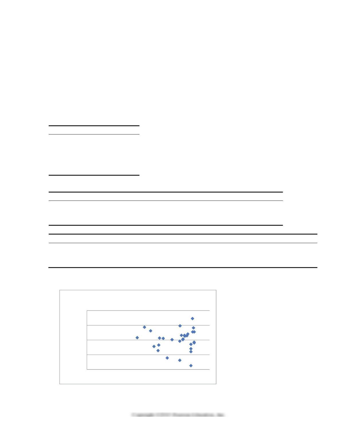
Introduction to Multiple Regression 14-63
SCENARIO 14-16
What are the factors that determine the acceleration time (in sec.) from 0 to 60 miles per hour of a
car? Data on the following variables for 30 different vehicle models were collected:
Y (Accel Time): Acceleration time in sec.
X1 (Engine Size): c.c.
X2 (Sedan): 1 if the vehicle model is a sedan and 0 otherwise
The regression results using acceleration time as the dependent variable and the remaining variables
as the independent variables are presented below.
Regression Statistics
Multiple R 0.6096
R Square 0.3716
Adjusted R Square 0.3251
Standard Error 1.4629
Observations 30
ANOVA
df SS MS F Significance F
Regression 2 34.1744 17.0872 7.9839 0.0019
Residual 27 57.7856 2.1402
Total 29 91.9600
Coefficients Standard Error t Stat P-value Lower 95% Upper 95%
Intercept 7.1052 0.6574 10.8086 0.0000 5.7564 8.4540
Engine Size -0.0005 0.0001 -3.6477 0.0011 -0.0008 -0.0002
Sedan 0.7264 0.5564 1.3056 0.2027 -0.4152 1.8681
The various residual plots are as shown below.
-4
-2
0
2
4
02468
Residuals
Predicted Y
Residuals versus Predicted Y
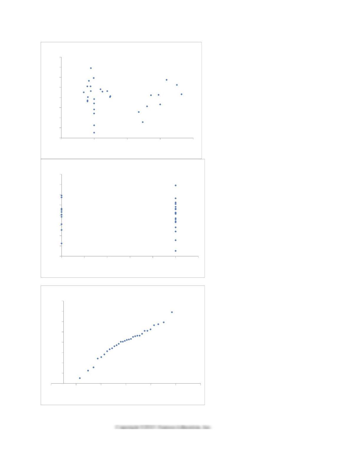
14-64 Introduction to Multiple Regression
-4
-3
-2
-1
0
1
2
3
4
0 2000 4000 6000 8000
Residuals
Engine
Residual Plot for Engine Size
-4
-3
-2
-1
0
1
2
3
4
0 0.2 0.4 0.6 0.8 1 1.2
Residuals
Sedan
Residual Plot for Sedan
-4
-3
-2
-1
0
1
2
3
4
-3 -2 -1 0 1 2 3
Residual
Z Value
Normal Probability Plot
Introduction to Multiple Regression 14-65
The coefficient of partial determinations 2
12Y
r⋅ and 2
21Y
r⋅are 0.3301, and 0.0594, respectively.
The coefficient of determination for the regression model using each of the 2 independent variables as
the dependent variable and the other independent variable as independent variables ( 2
j
R) are,
respectively 0.0077, and 0.0077.
240. Referring to Scenario 14-16, what is the correct interpretation for the estimated coefficient for
X1?
a) As the 0 to 60 miles per hour acceleration time increases by one second, the mean engine
size will decrease by an estimated 0.0005 c.c. without taking into consideration the other
independent variable included in the model.
b) As the engine size increases by one c.c., the mean 0 to 60 miles per hour acceleration
time will decrease by an estimated 0.0005 seconds without taking into consideration the
other independent variable included in the model.
c) As the 0 to 60 miles per hour acceleration time increases by one second, the mean engine
size will decrease by an estimated 0.0005 c.c. taking into consideration the other
independent variable included in the model.
d) As the engine size increases by one c.c., the mean 0 to 60 miles per hour acceleration
time will decrease by an estimated 0.0005 seconds taking into consideration the other
independent variable included in the model.
241. Referring to Scenario 14-16, what is the correct interpretation for the estimated coefficient for
X2?
a) The mean 0 to 60 miles per hour acceleration time of a sedan is estimated to be 0.7264
seconds lower than that of a non-sedan after considering the effect of the engine size.
b) The mean 0 to 60 miles per hour acceleration time of a sedan is estimated to be 0.7264
seconds higher than that of a non-sedan after considering the effect of the engine size.
c) The mean 0 to 60 miles per hour acceleration time of a sedan is estimated to be 0.7264
seconds lower than that of a non-sedan without considering the effect of the engine size.
d) The mean 0 to 60 miles per hour acceleration time of a sedan is estimated to be 0.7264
seconds higher than that of a non-sedan without considering the effect of the engine size.
242. True or False: Referring to Scenario 14-16, the 0 to 60 miles per hour acceleration time of a
sedan is predicted to be 0.7264 seconds higher than that of a non-sedan with the same engine size.
14-66 Introduction to Multiple Regression
243. True or False: Referring to Scenario 14-16, the 0 to 60 miles per hour acceleration time of a
sedan is predicted to be 0.7264 seconds lower than that of a non-sedan with the same engine size.
244. True or False: Referring to Scenario 14-16, the 0 to 60 miles per hour acceleration time of a
sedan is predicted to be 0.0005 seconds higher than that of a non-sedan with the same engine size.
245. True or False: Referring to Scenario 14-16, the 0 to 60 miles per hour acceleration time of a
sedan is predicted to be 0.0005 seconds lower than that of a non-sedan with the same engine size.
246. Referring to Scenario 14-16, what is the value of the test statistic to determine whether engine
size makes a significant contribution to the regression model in the presence of the other
independent variable at a 5% level of significance?
247. Referring to Scenario 14-16, what is the p-value of the test statistic to determine whether
engine size makes a significant contribution to the regression model in the presence of the other
independent variable at a 5% level of significance?
Introduction to Multiple Regression 14-67
248. True or False: Referring to Scenario 14-16, there is enough evidence to conclude that engine
size makes a significant contribution to the regression model in the presence of the other
independent variable at a 5% level of significance.
249. Referring to Scenario 14-16, what is the value of the test statistic to determine whether being a
sedan or not makes a significant contribution to the regression model in the presence of the other
independent variable at a 5% level of significance?
250. Referring to Scenario 14-16, what is the p-value of the test statistic to determine whether being
a sedan or not makes a significant contribution to the regression model in the presence of the
other independent variable at a 5% level of significance?
251. True or False: Referring to Scenario 14-16, there is enough evidence to conclude that being a
sedan or not makes a significant contribution to the regression model in the presence of the other
independent variable at a 5% level of significance.
252. Referring to Scenario 14-16, ________ of the variation in Accel Time can be explained by the
two independent variables after taking into consideration the number of independent variables
and the number of observations.
14-68 Introduction to Multiple Regression
253. Referring to Scenario 14-16, ________ of the variation in Accel Time can be explained by the
two independent variables.
254. Referring to Scenario 14-16, ________ of the variation in Accel Time can be explained by
engine size while controlling for the other independent variable.
255. Referring to Scenario 14-16, ________ of the variation in Accel Time can be explained by the
dummy variable Sedan while controlling for the other independent variable.
256. Referring to Scenario 14-16, which of the following assumptions is most likely violated based
on the residual plot of the residuals versus predicted Y?
a) Independence of errors.
b) Normality of errors.
c) Equal variance.
d) None.
257. Referring to Scenario 14-16, which of the following assumptions is most likely violated based
on the residual plot for Engine Size?
a) Linearity.
b) Normality of errors.
c) Independence of errors.
d) None.
Introduction to Multiple Regression 14-69
258. Referring to Scenario 14-16, which of the following assumptions is most likely violated based
on the normal probability plot?
a) Linearity.
b) Normality.
c) Equal variance.
d) Independence.
259. True or False: Referring to Scenario 14-16, the error appears to be left-skewed.
260. True or False: Referring to Scenario 14-16, the errors (residuals) appear to be right-skewed.

14-70 Introduction to Multiple Regression
SCENARIO 14-17
Given below are results from the regression analysis where the dependent variable is the number of
weeks a worker is unemployed due to a layoff (Unemploy) and the independent variables are the age
of the worker (Age) and a dummy variable for management position (Manager: 1 = yes, 0 = no).
The results of the regression analysis are given below:
Regression Statistics
Multiple R 0.6391
R Square 0.4085
Adjusted R Square 0.3765
Standard Error 18.8929
Observations 40
ANOVA
df SS MS F Significance F
Regression 2 9119.0897 4559.5448 12.7740 0.0000
Residual 37 13206.8103 356.9408
Total 39 22325.9
Coefficients Standard Error t Stat P-value
Intercept -0.2143 11.5796 -0.0185 0.9853
Age 1.4448 0.3160 4.5717 0.0000
Manager -22.5761 11.3488 -1.9893 0.0541
261. Referring to Scenario 14-17, which of the following is a correct statement?
a) On average, a worker who is a year older is estimated to stay jobless shorter by
approximately 0.2143 weeks while holding constant the effects of the manager dummy
variable.
b) On average, a worker who is a year older is estimated to stay jobless longer by
approximately 0.2143 weeks while holding constant the effects of the manager dummy
variable.
c) On average, a worker who is a year older is estimated to stay jobless shorter by
approximately 1.4448 weeks while holding constant the effects of the manager dummy
variable.
d) On average, a worker who is a year older is estimated to stay jobless longer by
approximately 1.4448 weeks while holding constant the effects of the manager dummy
variable.
Introduction to Multiple Regression 14-71
262. Referring to Scenario 14-17, which of the following is a correct statement?
a) On average, those who are in a management position are estimated to stay jobless shorter
by approximately 1.4448 weeks while holding constant the effects of age.
b) On average, those who are in a management position are estimated to stay jobless longer
by approximately 1.4448 weeks while holding constant the effects of age.
c) On average, those who are in a management position are estimated to stay jobless shorter
by approximately 22.5761 weeks while holding constant the effects of age.
d) On average, those who are in a management position are estimated to stay jobless longer
by approximately 22.5761 weeks while holding constant the effects of age.
263. Referring to Scenario 14-17, which of the following is a correct statement?
a) 40.85% of the total variation in the number of weeks a worker is unemployed due to a
layoff can be explained by the age of the worker and whether the worker is a manager.
b) 40.85% of the total variation in the number of weeks a worker is unemployed due to a
layoff can be explained by the age of the worker and whether the worker is a manager
after adjusting for the number of predictors and sample size.
c) 40.85% of the total variation in the number of weeks a worker is unemployed due to a
layoff can be explained by the age of the worker and whether the worker is a manager
after adjusting for the level of significance
d) 40.85% of the total variation in the number of weeks a worker is unemployed due to a
layoff can be explained by the age of the worker and whether the worker is a manager
holding constant the effect of all the independent variables.
264. Referring to Scenario 14-17, which of the following is a correct statement?
a) 37.65% of the total variation in the number of weeks a worker is unemployed due to a
layoff can be explained by the age of the worker and whether the worker is a manager.
b) 37.65% of the total variation in the number of weeks a worker is unemployed due to a
layoff can be explained by the age of the worker and whether the worker is a manager
after adjusting for the number of predictors and sample size.
c) 37.65% of the total variation in the number of weeks a worker is unemployed due to a
layoff can be explained by the age of the worker and whether the worker is a manager
after adjusting for the level of significance
d) 37.65% of the total variation in the number of weeks a worker is unemployed due to a
layoff can be explained by the age of the worker and whether the worker is a manager
holding constant the effect of all the independent variables.
14-72 Introduction to Multiple Regression
265. Referring to Scenario 14-17, what is the standard error of estimate?
266. Referring to Scenario 14-17, predict the number of weeks being unemployed due to a layoff for
a worker who is a thirty-year old and is a manager.
267. Referring to Scenario 14-17, estimate the mean number of weeks being unemployed due to a
layoff for a worker who is a thirty-year old and is a manager.
268. Referring to Scenario 14-17, which of the following is the correct null hypothesis to test
whether age has any effect on the number of weeks a worker is unemployed due to a layoff while
holding constant the effect of the other independent variable?
a) 01
:0H
β
=
b) 01
:0H
β
≠
c) 02
:0H
β
=
d) 02
:0H
β
≠
269. Referring to Scenario 14-17, which of the following is the correct alternative hypothesis to test
whether age has any effect on the number of weeks a worker is unemployed due to a layoff while
holding constant the effect of the other independent variable?
a) 11
:0H
β
=
b) 11
:0H
β
≠
c) 12
:0H
β
=
d) 12
:0H
β
≠
Introduction to Multiple Regression 14-73
270. Referring to Scenario 14-17, what is the value of the test statistic when testing whether age has
any effect on the number of weeks a worker is unemployed due to a layoff while holding constant
the effect of the other independent variable?
271. Referring to Scenario 14-17, what is the p-value of the test statistic when testing whether age
has any effect on the number of weeks a worker is unemployed due to a layoff while holding
constant the effect of the other independent variable?
272. True or False: Referring to Scenario 14-17, the null hypothesis should be rejected at a 10%
level of significance when testing whether age has any effect on the number of weeks a worker is
unemployed due to a layoff while holding constant the effect of the other independent variable.
273. True or False: Referring to Scenario 14-17, there is sufficient evidence that age has an effect on
the number of weeks a worker is unemployed due to a layoff while holding constant the effect of
the other independent variable at a 10% level of significance.
274. Referring to Scenario 14-17, which of the following is the correct null hypothesis to determine
whether there is a significant relationship between the number of weeks a worker is unemployed
due to a layoff and the entire set of explanatory variables?
a) 00 1 2
:0H
β
ββ
===
b) 01 2
:0H
β
β
==
c) 00 1 2
:H
β
ββ
==
d) 01 2
:H
ββ
=
14-74 Introduction to Multiple Regression
275. Referring to Scenario 14-17, which of the following is the correct alternative hypothesis to
determine whether there is a significant relationship between percentage of students passing the
proficiency test and the entire set of explanatory variables?
e) 1:
H
All 0
j
β
≠ for j = 0, 1, 2
f) 1:
H
All 0
j
β
≠ for j = 1, 2
g) 1:
H
At least one of 0
j
β
≠ for j = 0, 1, 2
h) 1:
H
At least one of 0
j
β
≠ for j = 1, 2
276. Referring to Scenario 14-17, the null hypothesis 01 2
:0H
β
β
==
implies that the number of
weeks a worker is unemployed due to a layoff is not affected by any of the explanatory variables.
277. Referring to Scenario 14-17, the null hypothesis 01 2
:0H
β
β
==
implies that the number of
weeks a worker is unemployed due to a layoff is not affected by some of the explanatory
variables.
278. Referring to Scenario 14-17, the null hypothesis 01 2
:0H
ββ
==
implies that the number of
weeks a worker is unemployed due to a layoff is not related to any of the explanatory variables.
279. Referring to Scenario 14-17, the null hypothesis 01 2
:0H
ββ
==
implies that the number of
weeks a worker is unemployed due to a layoff is not related to one of the explanatory variables.
Introduction to Multiple Regression 14-75
280. Referring to Scenario 14-17, the alternative hypothesis 1:
H
At least one of 0
j
β
≠ for j = 1, 2
implies that the number of weeks a worker is unemployed due to a layoff is related to all of the
explanatory variables.
281. Referring to Scenario 14-17, the alternative hypothesis 1:
H
At least one of 0
j
β
≠ for j = 1, 2
implies that the number of weeks a worker is unemployed due to a layoff is related to at least one
of the explanatory variables.
282. Referring to Scenario 14-17, the alternative hypothesis 1:
H
At least one of 0
j
β
≠ for j = 1, 2
implies that the number of weeks a worker is unemployed due to a layoff is affected by all of the
explanatory variables.
283. Referring to Scenario 14-17, the alternative hypothesis 1:
H
At least one of 0
j
β
≠ for j = 1, 2
implies that the number of weeks a worker is unemployed due to a layoff is affected by at least
one of the explanatory variables.
284. Referring to Scenario 14-17, what are the numerator and denominator degrees of freedom,
respectively, for the test statistic to determine whether there is a significant relationship between
the number of weeks a worker is unemployed due to a layoff and the entire set of explanatory
variables?
14-76 Introduction to Multiple Regression
285. Referring to Scenario 14-17, what is the value of the test statistic to determine whether there is
a significant relationship between the number of weeks a worker is unemployed due to a layoff
and the entire set of explanatory variables?
286. Referring to Scenario 14-17, what is the p-value of the test statistic to determine whether there
is a significant relationship between the number of weeks a worker is unemployed due to a layoff
and the entire set of explanatory variables?
287. True or False: Referring to Scenario 14-17, the null hypothesis should be rejected at a 10%
level of significance when testing whether there is a significant relationship between the number
of weeks a worker is unemployed due to a layoff and the entire set of explanatory variables.
288. True or False: Referring to Scenario 14-17, there is sufficient evidence that at least one of the
explanatory variables is related to the number of weeks a worker is unemployed due to a layoff at
a 10% level of significance.
289. True or False: Referring to Scenario 14-17, there is sufficient evidence that the number of
weeks a worker is unemployed due to a layoff depends on at least one of the explanatory
variables at a 10% level of significance.
290. True or False: Referring to Scenario 14-17, there is sufficient evidence that all of the
explanatory variables are related to the number of weeks a worker is unemployed due to a layoff
at a 10% level of significance.
291. True or False: Referring to Scenario 14-17, there is sufficient evidence that the number of
weeks a worker is unemployed due to a layoff depends on all of the explanatory variables at a
10% level of significance.
292. Referring to Scenario 14-17, what are the lower and upper limits of the 95% confidence
interval estimate for the effect of a one year increase in age on the mean number of weeks a
worker is unemployed due to a layoff after taking into consideration the effect of all the other
independent variables?
293. Referring to Scenario 14-17, what are the lower and upper limits of the 95% confidence
interval estimate for the difference in the mean number of weeks a worker is unemployed due to a
layoff between a worker who is in a management position and one who is not after taking into
consideration the effect of all the other independent variables?
294. True or False: Referring to Scenario 14-17, you can conclude that, holding constant the effect
of the other independent variable, age has no impact on the mean number of weeks a worker is
unemployed due to a layoff at a 5% level of significance if we use only the information of the
95% confidence interval estimate for the effect of a one year increase in age on the mean number
of weeks a worker is unemployed due to a layoff.
14-78 Introduction to Multiple Regression
295. True or False: Referring to Scenario 14-17, we can conclude that, holding constant the effect of
the other independent variable, there is a difference in the mean number of weeks a worker is
unemployed due to a layoff between a worker who is in a management position and one who is
not at a 5% level of significance if we use only the information of the 95% confidence interval
estimate for the difference in the mean number of weeks a worker is unemployed due to a layoff
between a worker who is in a management position and one who is not.
296. True or False: Referring to Scenario 14-17, we can conclude definitively that, holding constant
the effect of the other independent variable, age has no impact on the mean number of weeks a
worker is unemployed due to a layoff at a 1% level of significance if all we have is the
information of the 95% confidence interval estimate for the effect of a one year increase in age on
the mean number of weeks a worker is unemployed due to a layoff.
297. True or False: Referring to Scenario 14-17, we can conclude definitively that, holding constant
the effect of the other independent variables, there is not a difference in the mean number of
weeks a worker is unemployed due to a layoff between a worker who is in a management position
and one who is not at a 1% level of significance if all we have is the information of the 95%
confidence interval estimate for the difference in the mean number of weeks a worker is
unemployed due to a layoff between a worker who is in a management position and one who is
not.
Introduction to Multiple Regression 14-79
298. True or False: Referring to Scenario 14-17, we can conclude definitively that, holding constant
the effect of the other independent variable, age has an impact on the mean number of weeks a
worker is unemployed due to a layoff at a 10% level of significance if all we have is the
information of the 95% confidence interval estimate for the effect of a one year increase in age on
the mean number of weeks a worker is unemployed due to a layoff.
299. True or False: Referring to Scenario 14-17, we can conclude definitively that, holding constant
the effect of the other independent variables, there is not a difference in the mean number of
weeks a worker is unemployed due to a layoff between a worker who is in a management position
and one who is not at a 10% level of significance if all we have is the information of the 95%
confidence interval estimate for the difference in the mean number of weeks a worker is
unemployed due to a layoff between a worker who is in a management position and one who is
not.
14-80 Introduction to Multiple Regression
SCENARIO 14-18
A logistic regression model was estimated in order to predict the probability that a randomly chosen
university or college would be a private university using information on mean total Scholastic
Aptitude Test score (SAT) at the university or college and whether the TOEFL criterion is at least 90
(Toefl90 = 1 if yes, 0 otherwise.) The dependent variable, Y, is school type (Type = 1 if private and
0 otherwise).
The PHStat output is given below:
Binary Logistic Regression
Predictor Coefficients SE Coef Z p-Value
Intercept -3.9594 1.6741 -2.3650 0.0180
SAT 0.0028 0.0011 2.5459 0.0109
Toefl90:1 0.1928 0.5827 0.3309 0.7407
Deviance 101.9826
300. Referring to Scenario 14-18, which of the following is the correct expression for the estimated
model?
a) 3.9594 0.0028 0.1928 90YSATToefl=− + +
b) ˆ3.9594 0.0028 0.1928 90YSATToefl=− + +
c)
()
ln odds ratio 3.9594 0.0028 0.1928 90SAT Toefl=− + +
d)
()
ln estimated odds ratio 3.9594 0.0028 0.1928 90SAT Toefl=− + +
301. Referring to Scenario 14-18, what is the estimated odds ratio for a school with a mean SAT
score of 1250 and a TOEFL criterion that is at least 90?
302. Referring to Scenario 14-18, what is the estimated probability that a school with a mean SAT
score of 1250 and a TOEFL criterion that is at least 90?
Introduction to Multiple Regression 14-81
303. Referring to Scenario 14-18, what is the estimated odds ratio for a school with a mean SAT
score of 1100 and a TOEFL criterion that is not at least 90?
304. Referring to Scenario 14-18, what is the estimated probability that a school with a mean SAT
score of 1100 and a TOEFL criterion that is not at least 90?
305. Referring to Scenario 14-18, which of the following is the correct interpretation for the SAT
slope coefficient?
a) Holding constant the effect of Toefl90, the estimated mean value of school type increases
by 0.0028 for each increase of one point in average SAT score.
b) Holding constant the effect of Toefl90, the estimated school type increases by 0.0028 for
each increase of one point in average SAT score.
c) Holding constant the effect of Toefl90, the estimated probability of the school being a
private school increases by 0.0028 for each increase of one point in mean SAT score.
d) Holding constant the effect of Toefl90, the estimated natural logarithm of the odds ratio
of the school being a private school increases by 0.0028 for each increase of one point in
mean SAT score.
306. Referring to Scenario 14-18, which of the following is the correct interpretation for the Toefl90
slope coefficient?
a) Holding constant the effect of SAT, the estimated mean value of school type is 0.1928
higher when the school has a TOEFL criterion that is at least 90.
b) Holding constant the effect of SAT, the estimated school type increases by 0.1928 when
the school has a TOEFL criterion that is at least 90.
c) Holding constant the effect of SAT, the estimated natural logarithm of the odds ratio of
the school being a private school is 0.1928 higher for a school that has a TOEFL criterion
that is at least 90 than one that does not.
d) Holding constant the effect of SAT, the estimated probability of the school being a
private school is 0.1928 higher for a school that has a TOEFL criterion that is at least 90
than one that does not.
14-82 Introduction to Multiple Regression
307. Referring to Scenario 14-18, what are the degrees of freedom for the chi-square distribution
when testing whether the model is a good-fitting model?
308. Referring to Scenario 14-18, what is the p-value of the test statistic when testing whether the
model is a good-fitting model?
309. True or False: Referring to Scenario 14-18, the null hypothesis that the model is a good-fitting
model cannot be rejected when allowing for a 5% probability of making a type I error.
310. True or False: Referring to Scenario 14-18, there is not enough evidence to conclude that the
model is not a good-fitting model at a 0.05 level of significance.
311. Referring to Scenario 14-18, what is the p-value of the test statistic when testing whether SAT
makes a significant contribution to the model in the presence of Toefl90?
312. Referring to Scenario 14-18, what should be the decision (‘reject’ or ‘do not reject’) on the null
hypothesis when testing whether SAT makes a significant contribution to the model in the
presence of Toefl90 at a 0.05 level of significance?
Introduction to Multiple Regression 14-83
313. True or False: Referring to Scenario 14-18, there is not enough evidence to conclude that SAT
score makes a significant contribution to the model in the presence of Toefl90 at a 0.05 level of
significance.
314. Referring to Scenario 14-18, what is the p-value of the test statistic when testing whether
Toefl90 makes a significant contribution to the model in the presence of SAT?
315. Referring to Scenario 14-18, what should be the decision (‘reject’ or ‘do not reject’) on the null
hypothesis when testing whether Toefl90 makes a significant contribution to the model in the
presence of SAT at a 0.05 level of significance?
316. True or False: Referring to Scenario 14-18, there is not enough evidence to conclude that
Toefl90 makes a significant contribution to the model in the presence of SAT at a 0.05 level of
significance.
14-84 Introduction to Multiple Regression
SCENARIO 14-19
The marketing manager for a nationally franchised lawn service company would like to study the
characteristics that differentiate home owners who do and do not have a lawn service. A random
sample of 30 home owners located in a suburban area near a large city was selected; 11 did not have
a lawn service (code 0) and 19 had a lawn service (code 1). Additional information available
concerning these 30 home owners includes family income (Income, in thousands of dollars) and lawn
size (Lawn Size, in thousands of square feet).
The PHStat output is given below:
Binary Logistic Regression
Predictor Coefficients SE Coef Z p-Value
Intercept -7.8562 3.8224 -2.0553 0.0398
Income 0.0304 0.0133 2.2897 0.0220
Lawn Size 1.2804 0.6971 1.8368 0.0662
Deviance 25.3089
317. Referring to Scenario 14-19, which of the following is the correct expression for the estimated
model?
a) 7.8562 0.0304 1.2804 Y Income LawnSize=− + +
b) ˆ7.8562 0.0304 1.2804 Y Income LawnSize=− + +
c)
()
ln odds ratio 7.8562 0.0304 1.2804 Income LawnSize=− + +
d)
()
ln estimated odds ratio 7.8562 0.0304 1.2804 Income LawnSize=− + +
318. Referring to Scenario 14-19, what is the estimated odds ratio for a home owner with a family
income of $100,000 and a lawn size of 5,000 square feet?
319. Referring to Scenario 14-19, what is the estimated probability that a home owner with a family
income of $100,000 and a lawn size of 5,000 square feet will purchase a lawn service?
Introduction to Multiple Regression 14-85
320. Referring to Scenario 14-19, what is the estimated odds ratio for a home owner with a family
income of $50,000 and a lawn size of 5,000 square feet?
321. Referring to Scenario 14-19, what is the estimated probability that a home owner with a family
income of $50,000 and a lawn size of 5,000 square feet will purchase a lawn service?
322. Referring to Scenario 14-19, what is the estimated odds ratio for a home owner with a family
income of $50,000 and a lawn size of 2,000 square feet?
323. Referring to Scenario 14-19, what is the estimated probability that a home owner with a family
income of $50,000 and a lawn size of 2,000 square feet will purchase a lawn service?
324. Referring to Scenario 14-19, what is the estimated odds ratio for a home owner with a family
income of $100,000 and a lawn size of 2,000 square feet?
325. Referring to Scenario 14-19, what is the estimated probability that a home owner with a family
income of $100,000 and a lawn size of 2,000 square feet will purchase a lawn service?
14-86 Introduction to Multiple Regression
326. Referring to Scenario 14-19, which of the following is the correct interpretation for the Income
slope coefficient?
a) Holding constant the effect of lawn size, the estimated number of lawn service purchased
increases by 0.0304 for each increase of one thousand dollars in family income.
b) Holding constant the effect of lawn size, the estimated average number of lawn service
purchased increases by 0.0304 for each increase of one thousand dollars in family
income.
c) Holding constant the effect of lawn size, the estimated probability of purchasing a lawn
service increases by 0.0304 for each increase of one thousand dollars in family income.
d) Holding constant the effect of lawn size, the estimated natural logarithm of the odds ratio
of purchasing a lawn service increases by 0.0304 for each increase of one thousand
dollars in family income.
327. Referring to Scenario 14-19, which of the following is the correct interpretation for the Lawn
Size slope coefficient?
a) Holding constant the effect of income, the estimated number of lawn service purchased
increases by 1.2804 for each increase of one thousand square feet in lawn size.
b) Holding constant the effect of income, the estimated average number of lawn service
purchased increases by 1.2804 for each increase of one thousand square feet in lawn size.
c) Holding constant the effect of income, the estimated probability of purchasing a lawn
service increases by 1.2804 for each increase of one thousand square feet in lawn size.
d) Holding constant the effect of income, the estimated natural logarithm of the odds ratio of
purchasing a lawn service increases by 1.2804 for each increase of one thousand square
feet in lawn size.
328. Referring to Scenario 14-19, what are the degrees of freedom for the chi-square distribution
when testing whether the model is a good-fitting model?
Introduction to Multiple Regression 14-87
329. Referring to Scenario 14-19, what is the p-value of the test statistic when testing whether the
model is a good-fitting model?
330. True or False: Referring to Scenario 14-19, the null hypothesis that the model is a good-fitting
model cannot be rejected when allowing for a 5% probability of making a type I error.
331. True or False: Referring to Scenario 14-19, there is not enough evidence to conclude that the
model is not a good-fitting model at a 0.05 level of significance.
332. Referring to Scenario 14-19, what is the p-value of the test statistic when testing whether
Income makes a significant contribution to the model in the presence of LawnSize?
333. Referring to Scenario 14-19, what should be the decision (‘reject’ or ‘do not reject’) on the null
hypothesis when testing whether Income makes a significant contribution to the model in the
presence of LawnSize at a 0.05 level of significance?
334. True or False: Referring to Scenario 14-19, there is not enough evidence to conclude that
Income makes a significant contribution to the model in the presence of LawnSize at a 0.05 level
of significance.
14-88 Introduction to Multiple Regression
335. Referring to Scenario 14-19, what is the p-value of the test statistic when testing whether
LawnSize makes a significant contribution to the model in the presence of Income?
336. Referring to Scenario 14-19, what should be the decision (‘reject’ or ‘do not reject’) on the null
hypothesis when testing whether LawnSize makes a significant contribution to the model in the
presence of Income at a 0.05 level of significance?
337. True or False: Referring to Scenario 14-19, there is not enough evidence to conclude that
LawnSize makes a significant contribution to the model in the presence of Income at a 0.05 level
of significance.
338. Which of the following is used to determine observations that have influential effect on the
fitted model?
a) Durbin Watson statistic
b) Variance inflationary factor
c) The Cp statistic
d) Cook’s distance statistic
339. Which of the following is NOT used to determine observations that have influential effect on
the fitted model?
a) The hat matrix elements hi
b) The studentized deleted residuals ti
c) The Cp statistic
d) Cook’s distance statistic
Introduction to Multiple Regression 14-89
340. Using the hat matrix elements hi to determine influential points in a multiple regression model
with k independent variable and n observations, Xi is an influential point if
a)
()
21/
i
hkn<+
b)
()
21/
i
hkn>+
c)
()
1/2
i
hnk<+
d)
()
1/2
i
hnk>+
341. Using the Studentized residuals ti to determine influential points in a multiple regression model
with k independent variable and n observations and letting tn-k-2 denote the upper critical value of
a two-tail t test with a 0.10 level of significance, Xi is an influential point if
a) 1ink
tt
−−
<
b) 1ink
tt
−−
>
c) 2ink
tt
−−
<
d) 2ink
tt
−−
>
342. Using the Cook’s distance statistic Di to determine influential points in a multiple regression
model with k independent variable and n observations and letting 12
,
F
ν
ν
denote the critical value of
an F distribution with 1
ν
and 2
ν
degrees of freedom at a 0.50 level of significance, Xi is an
influential point if
a) 1, 1iknk
DF
+−−
<
b) 1, 1iknk
DF
+−−
>
c) 1, 1inkk
DF
−− +
<
d) 1, 1inkk
DF
−− +
>

14-90 Introduction to Multiple Regression
343. True or False: Only when all three of the hat matrix elements hi, the Studentized deleted
residuals ti and the Cook’s distance statistic Di reveal consistent result should an observation be
removed from the regression analysis.