Chapter 13 – Queuing Models
1. Which of the following is not one of the important issues defining types of arrivals in a queuing system?
a.
Whether customers arrive one at a time or in batches.
b.
Whether customers are all essentially alike or are in separate priority classes.
c.
Whether customers have been through the system before or not
d.
Whether customers will wait in line or not
c
1
2. When a customer already in line in a queuing system becomes impatient and leaves the system before starting service,
this is called:
a.
balking
b.
limited waiting
c.
quitting
d.
reneging
d
1
3. Which of the following is not one of the types of service disciplines?
a.
Longest-processing-time
b.
First-come-first-served
c.
Service-in-random-order
d.
Last-come-first-served
a
1
4. A queuing system where customers join a single line and then are served by the first available server are said to be:
a.
in parallel
b.
in series
c.
random
d.
networked
a
1
5. A requirement for steady state analysis of a queuing system is that:
a.
the initial conditions are still in effect
b.
the waiting time must be exponentially distributed
c.
the analysis period is at least two hours
d.
the service rate must be constant
d
1
6. The exponential distribution is:
a.
flat
b.
bell-shaped
c.
heavily right-skewed
Chapter 13 – Queuing Models
d.
heavily left-skewed
c
1
7. The parameter λ in an exponential distribution can be interpreted as a:
a.
time
b.
rate
c.
mean
d.
standard deviation
b
1
8. Server utilization is the:
a.
amount of time a typical server is busy
b.
fraction of time a typical server is busy
c.
number of servers being used in a system
d.
number of times a server is used in a system
b
1
9. Traffic intensity is a very useful measure of:
a.
whether the system is stable or not
b.
the number of customers in a system
c.
the distribution of interarrival times
d.
the amount of congestion in the system
d
1
10. As the traffic intensity approaches 1:
a.
there is no waiting
b.
waiting lines stabilize
c.
waiting lines grow extremely rapidly
d.
at least one server will be idle
c
1
11. The two basic modeling approaches for queuing systems are optimization and simulation.
a.
True
b.
False
False
1
12. Almost all queuing systems are alike in that customers enter a system, possibly wait in one or more queues, get served,
and then depart.
a.
True
Chapter 13 – Queuing Models
b.
False
True
1
13. The decision to balk at entering a queuing system can be made by the customer or the system.
a.
True
b.
False
True
1
14. The mean and standard deviation of an exponential distribution are both equal to the parameter λ.
a.
True
b.
False
False
1
15. In a process where interarrival times are exponentially distributed, the time since the last arrival is irrelevant.
a.
True
b.
False
True
1
16. Exponentially distributed service times are often more realistic than exponentially distributed interarrival times.
a.
True
b.
False
False
1
17.
The server utilization U in an M/M/s system is always the same as the traffic intensity.
a.
True
b.
False
True
1
18. In queuing systems with a finite number of customers allowed, there is no need to require that the traffic intensity be
less than 1 to ensure stability.
a.
True
b.
False
True
1
19. In an Erlang loss model, customers who arrive when all servers are busy are lost to the system.
a.
True
b.
False
True
20. Congestion in a queuing system will be unaffected by changes in the variability of the interarrival time and service
time distributions, as long as the distributions retain the same means.
a.
True
b.
False
False
1
Exhibit 13-1
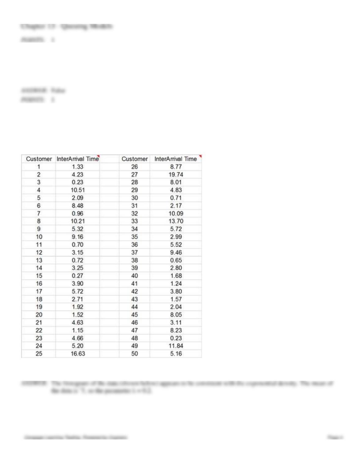
A grocery store manager would like to use an analytical queueing model to study the lines of customers that form in front
of the checkout stations in the store. During a period of time when business is steady, several store employees have
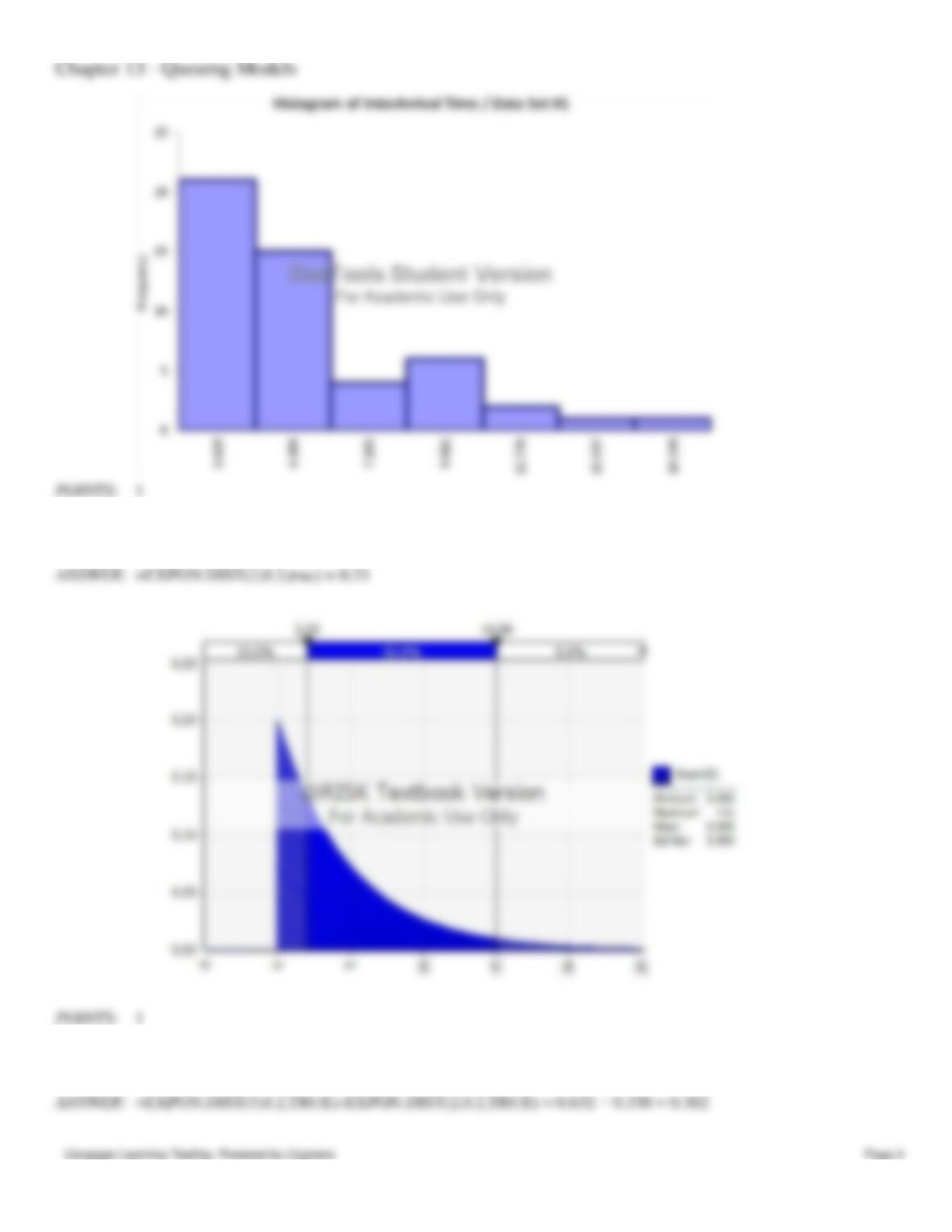
gathered data on customer interarrival times, which are shown below.
21. [Part 1] Refer to Exhibit 13–1. Is it reasonable to assume exponentially distributed interarrival times for the grocery
store customers? If so, what is λ?
1
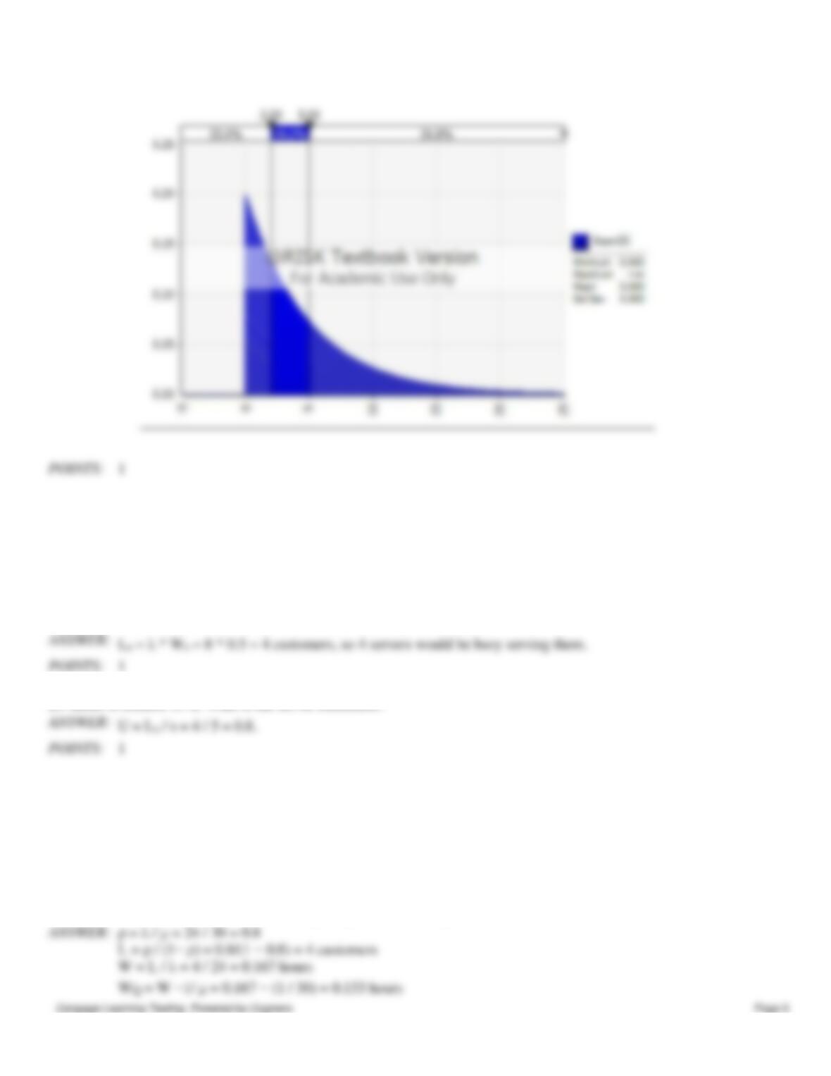
22. [Part 2] Refer to Exhibit 13–1. Assuming an exponential distribution with the parameter λ you obtained in Part 1,
what is the probability that a customer interarrival time will be less than 2 minutes?
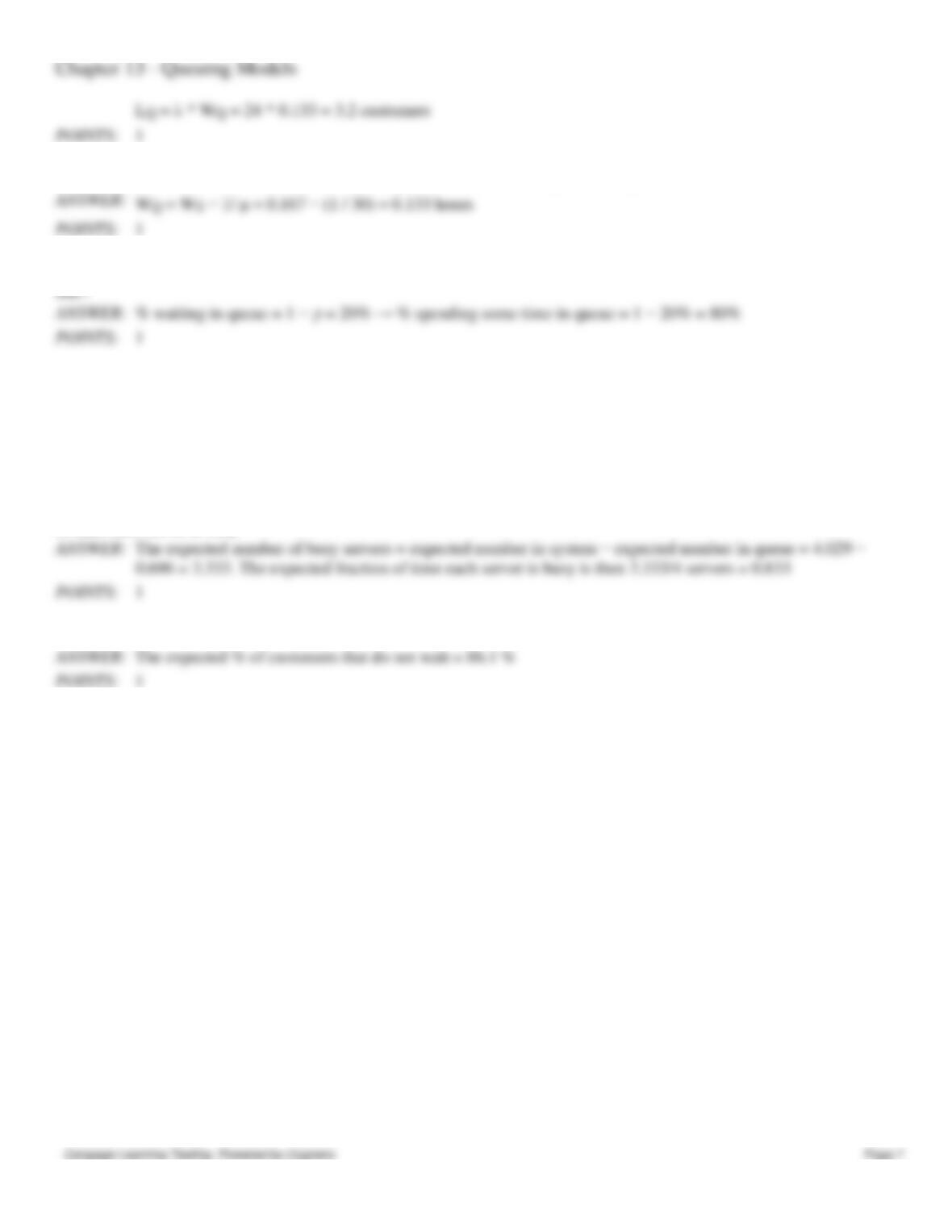
23. [Part 3] Refer to Exhibit 13–1. Again assuming an exponential distribution with the parameter λ you obtained in Part
2, what is the probability that a customer interarrival time will be more than 2 minutes, but less than 5 minutes?
Chapter 13 – Queuing Models
Exhibit 13-2
An oil-change facility serves customers that enter at a rate of 8 per hour. There are five servers available to perform oil
changes for entering customers. Customers wait in a single line and enter the facility, in first-come-first-serve fashion, to
the first of the five servers who is available. Each server can change the oil of one customer’s car every 30 minutes on
average.
24. Refer to Exhibit 13–2. How many of the servers are busy on average?
25. Refer to Exhibit 13–2. What is the server utilization?
Exhibit 13-3
A Credit Union has a small branch in which a single customer service representative serves the needs of customers who
arrive at an average rate of 24 per hour. The service representative can typically handle 30 customers per hour. Based on
an analysis of historical data, it is reasonable to assume that customer interarrival times and service times are
exponentially distributed. Assume that all arriving customers enter the branch, regardless of the number already waiting in
line.
26. Refer to Exhibit 13–3. What is the average length of the waiting line?
27. Refer to Exhibit 13–3. What is the average length of time (in hours) spent waiting in line?
% waiting in queue = 1 − ρ = 20% → % spending some time in queue = 1 − 20% = 80%
28. Refer to Exhibit 13–3. What percentage of all customers have to spend at least some small amount of time waiting in
Exhibit 13-4
Consider a fast-food restaurant where customers arrive at a Poisson rate of 100 per hour. Four equally capable servers
work at the restaurant during a typical hour of operation. Each employee takes, on average, 2 minutes to serve a customer,
and service times are exponentially distributed. Customers who arrive and find all 4 servers busy join a single queue and
are then served in first-come-first-served fashion.
29. Refer to Exhibit 13–4. Use the M/M/s template to find the expected number of busy servers, and the expected fraction
of time each server is busy
The expected number of busy servers = expected number in system − expected number in queue = 4.029 −
0.696 = 3.333. The expected fraction of time each server is busy is then 3.333/4 servers = 0.833
30. Refer to Exhibit 13–4. What percentage of customers do not wait in the queue?
The expected % of customers that do not wait = 86.1 %