Exam
Name___________________________________
SHORT ANSWER. Write the word or phrase that best completes each statement or answers the question.
Preliminary data analyses indicate that it is reasonable to consider the assumptions for one–way ANOVA satisfied.
Perform the required hypothesis test using the critical–value approach.
1)
At the 0.025 significance level, do the data provide sufficient evidence to conclude that a
difference exists between the population means of the four different brands? The sample
data are given below.
Brand A
17
20
21
22
21
Brand B
18
18
23
25
26
Brand C
21
24
25
26
29
29
Brand D
22
25
27
29
35
36
37
1)
2)
Four different types of fertilizers are used on raspberry plants. The number of raspberries
on each randomly selected plant is given below. Test the claim that the type of fertilizer
makes no difference in the mean number of raspberries per plant. Use = 0.01.
Fertilizer 1 Fertilizer 2 Fertilizer 3 Fertilizer 4
6 8 6 3
5 5 3 5
7 5 4 3
6 5 3 4
7 5 2 4
6 6 3 5
2)
Preliminary data analyses indicate that it is reasonable to consider the assumptions for one–way ANOVA satisfied. Use
Minitab to perform the required hypothesis test using the p–value approach.
3)
Random samples of four different models of cars were selected and the gas mileage of each
car was measured. The results are shown below.
Model A
23
25
24
26
Model B
28
26
29
30
Model C
30
28
32
27
Model D
25
26
25
28
Test the claim that the four different models have the same population mean. Use a
significance level of 0.05.
3)
4)
A consumer magazine wants to compare the lifetimes of ballpoint pens of three different
types. The magazine takes a random sample of pens of each type in the following table.
Brand 1
260
218
184
219
Brand 2
181
240
162
218
Brand 3
238
257
241
213
Do the data indicate that there is a difference in mean lifetime for the three brands of
ballpoint pens? Use = 0.01.
4)
Preliminary data analyses indicate that it is reasonable to consider the assumptions for one–way ANOVA satisfied.
Perform the required hypothesis test using the critical–value approach.
5)
A consumer magazine wants to compare the lifetimes of ballpoint pens of three different
types. The magazine takes a random sample of pens of each type in the following table.
Brand 1
260
218
184
219
Brand 2
181
240
162
218
Brand 3
238
257
241
213
Do the data indicate that there is a difference in mean lifetime for the three brands of
ballpoint pens? Use = 0.01.
5)
Provide an appropriate response.
6)
List the basic properties of F–curves.
6)
Preliminary data analyses indicate that it is reasonable to consider the assumptions for one–way ANOVA satisfied. Use
Minitab to perform the required hypothesis test using the p–value approach.
7)
At the 0.025 significance level, do the data provide sufficient evidence to conclude that a
difference exists between the population means of the four different brands? The sample
data are given below.
Brand A
15
25
21
23
22
20
Brand B
20
17
22
23
Brand C
21
22
20
19
18
Brand D
15
15
14
23
22
28
28
7)
8)
At the 0.01 significance level, do the data provide sufficient evidence to conclude that a
difference exists between the population means of the three different brands ? The sample
data are given below.
Brand A
44
47
44
40
39
Brand B
30
32
34
36
38
40
42
Brand C
28
27
31
32
36
8)
Provide an appropriate response.
9)
When performing a one–way ANOVA, two of the assumptions required are that the
populations be normally distributed and that the populations have equal standard
deviations. What rule of thumb can be used to assess the equal–standard deviations
assumption? What other method can be used to assess the normality and equal–standard
deviations assumptions?
9)
Preliminary data analyses indicate that it is reasonable to consider the assumptions for one–way ANOVA satisfied.
Perform the required hypothesis test using the critical–value approach.
10)
A medical researcher wishes to try three different techniques to lower blood pressure of
patients with high blood pressure. The subjects are randomly selected and assigned to one
of three groups. Group 1 is given medication, Group 2 is given an exercise program, and
Group 3 is assigned a diet program. At the end of six weeks, each subject’s blood pressure
is recorded. Test the claim that there is no difference among the means. Use = 0.05.
Group 1 Group 2 Group 3
984
12 212
11 5 4
15 3 6
13 4 9
808
10)
Provide an appropriate response.
11)
A one–way ANOVA is being performed. Suppose that SST =144.3 and SSE =71.8. Find the
value of the third sum of squares, give its notation, state its name and the source of
variation it represents.
11)
12)
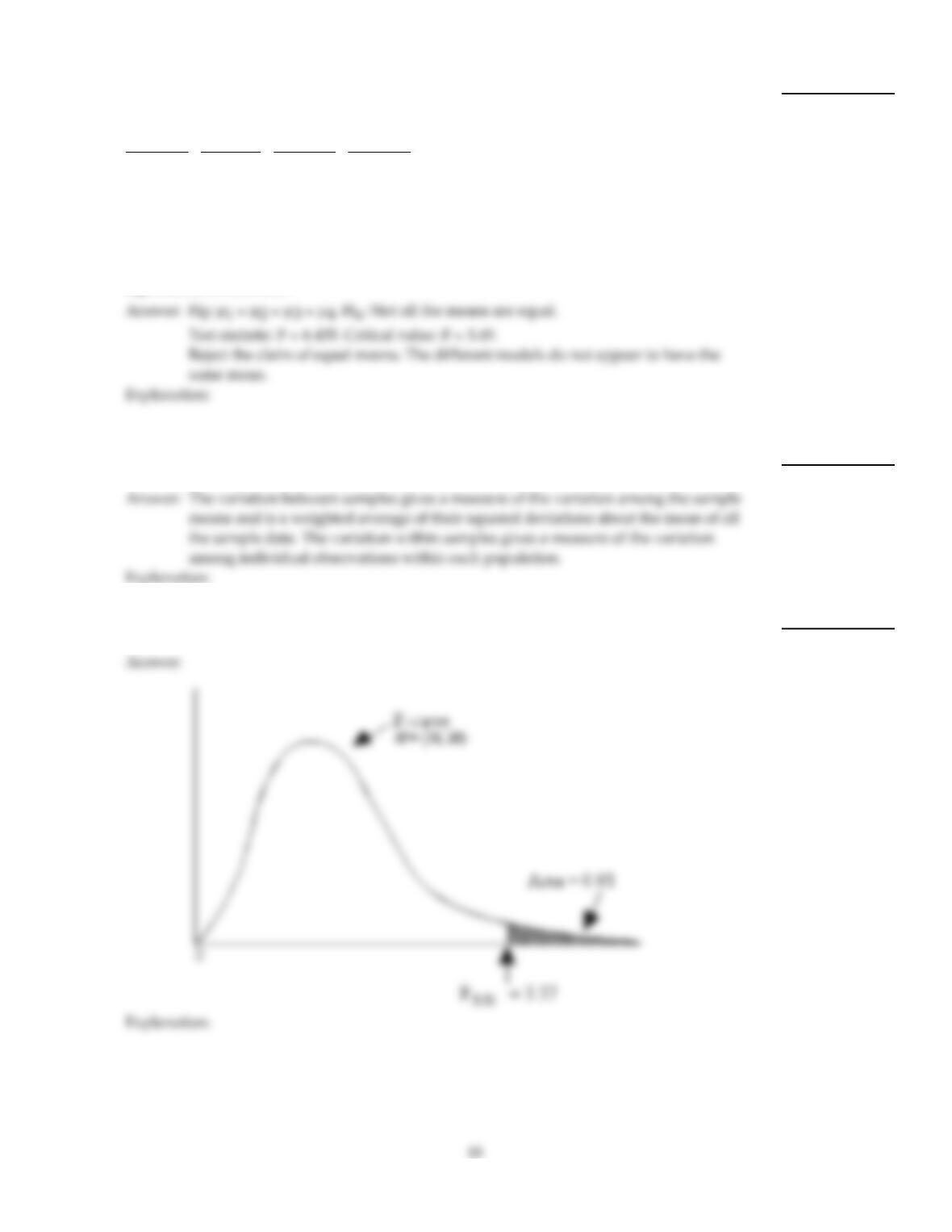
For an F–curve with df = (8, 3), find the F–value having area 0.05 to its right and illustrate
your answer with a sketch.
12)
Preliminary data analyses indicate that it is reasonable to consider the assumptions for one–way ANOVA satisfied.
Perform the required hypothesis test using the critical–value approach.
13)
At the 0.025 significance level, do the data provide sufficient evidence to conclude that a
difference exists between the population means of the four different brands? The sample
data are given below.
Brand A
15
25
21
23
22
20
Brand B
20
17
22
23
Brand C
21
22
20
19
18
Brand D
15
15
14
23
22
28
28
13)
Preliminary data analyses indicate that it is reasonable to consider the assumptions for one–way ANOVA satisfied. Use
Minitab to perform the required hypothesis test using the p–value approach.
14)
At the 0.025 significance level, do the data provide sufficient evidence to conclude that a
difference exists between the population means of the three different brands? The sample
data are given below.
Brand A
32
34
37
33
36
39
Brand B
27
24
33
30
Brand C
22
25
32
22
21
14)
Preliminary data analyses indicate that it is reasonable to consider the assumptions for one–way ANOVA satisfied.
Perform the required hypothesis test using the critical–value approach.
15)
The data below represent the weight losses for people on three different exercise programs.
Exercise A
2.5
8.8
7.3
9.8
5.1
Exercise B
5.8
4.9
1.1
7.8
1.2
Exercise C
4.3
6.2
5.8
8.1
7.9
At the 1% significance level, does it appear that a difference exists in the true mean weight
loss produced by the three exercise programs?
15)
Explanation:
Preliminary data analyses indicate that it is reasonable to consider the assumptions for one–way ANOVA satisfied. Use
Minitab to perform the required hypothesis test using the p–value approach.
16)
At the 0.025 significance level, do the data provide sufficient evidence to conclude that a
difference exists between the population means of the four different brands? The sample
data are given below.
Brand A
17
20
21
22
21
Brand B
18
18
23
25
26
Brand C
21
24
25
26
29
29
Brand D
22
25
27
29
35
36
37
16)
Explanation:
Preliminary data analyses indicate that it is reasonable to consider the assumptions for one–way ANOVA satisfied.
Perform the required hypothesis test using the critical–value approach.
17)
A realtor wishes to compare the square footage of houses in 4 different cities, all of which
are priced approximately the same. The data are listed below. Can the realtor conclude that
the mean square footage in the four cities are equal? Use = 0.01.
City #1 City #2 City #3 City #4
2150 1780 1530 2400
1980 1540 1600 2350
2210 1690 1580 2600
2000 1650 1750 2150
1900 1500 2000
1670 2200
2350
17)
Provide an appropriate response.
18)
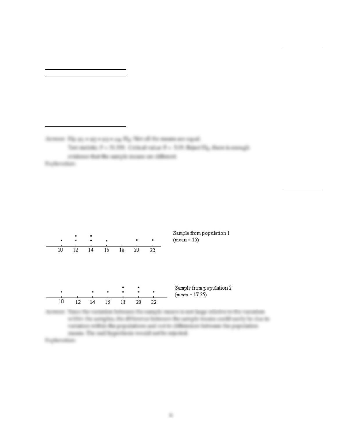
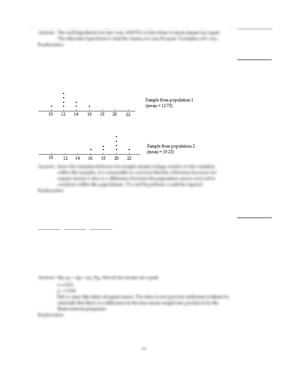
A one–way ANOVA is to be performed. Independent random samples are taken from two
populations. The sample data are depicted in the dotplot below. Is it reasonable to
conclude that the difference between the sample means is due to a difference between the
population means and not to variation within the populations? Do you think the null
hypothesis would be rejected? Explain your thinking.
18)
Preliminary data analyses indicate that it is reasonable to consider the assumptions for one–way ANOVA satisfied.
Perform the required hypothesis test using the critical–value approach.
19)
At the 0.01 significance level, do the data provide sufficient evidence to conclude that a
difference exists between the population means of the three different brands ? The sample
data are given below.
Brand A
44
47
44
40
39
Brand B
30
32
34
36
38
40
42
Brand C
28
27
31
32
36
19)
Provide an appropriate response.
20)
A one–way ANOVA is being performed. Suppose that SST =82.1 and SSTR =55.6. Find
the value of the third sum of squares, give its notation, state its name and the source of
variation it represents.
20)
Preliminary data analyses indicate that it is reasonable to consider the assumptions for one–way ANOVA satisfied.
Perform the required hypothesis test using the critical–value approach.
21)
At the 0.025 significance level, do the data provide sufficient evidence to conclude that a
difference exists between the population means of the three different brands? The sample
data are given below.
Brand A
32
34
37
33
36
39
Brand B
27
24
33
30
Brand C
22
25
32
22
21
21)
22)
Random samples of four different models of cars were selected and the gas mileage of each
car was measured. The results are shown below.
Model A
23
25
24
26
Model B
28
26
29
30
Model C
30
28
32
27
Model D
25
26
25
28
Test the claim that the four different models have the same population mean. Use a
significance level of 0.05.
22)
Provide an appropriate response.
23)
In the context of a one–way ANOVA, explain what is meant by variation between samples
and variation within samples.
23)
24)
For an F–curve with df = (10, 20), find the F–value having area 0.01 to its right and
illustrate your answer with a sketch.
24)
25)
Describe the null and alternate hypotheses for one–way ANOVA. Give an example.
25)
26)
A one–way ANOVA is to be performed. Independent random samples are taken from two
populations. The sample data are depicted in the dotplot below. Is it reasonable to
conclude that the difference between the sample means is due to a difference between the
population means and not to variation within the populations? Do you think the null
hypothesis would be rejected? Explain your thinking.
26)
Preliminary data analyses indicate that it is reasonable to consider the assumptions for one–way ANOVA satisfied. Use
Minitab to perform the required hypothesis test using the p–value approach.
27)
The data below represent the weight losses for people on three different exercise programs.
Exercise A
2.5
8.8
7.3
9.8
5.1
Exercise B
5.8
4.9
1.1
7.8
1.2
Exercise C
4.3
6.2
5.8
8.1
7.9
At the 1% significance level, does it appear that a difference exists in the true mean weight
loss produced by the three exercise programs?
27)
Provide an appropriate response.
28)
A one–way ANOVA is to be performed. The following sample data are obtained.
x1= 20, x2= 30, x3= 40
The common population standard deviation for the three populations is 2.5. Do you think
that the difference between the sample means could be due to variation within the
populations or does it seem clear that the difference between the sample means is due to a
difference between population means? Do you think that the null hypothesis would be
rejected? Explain your thinking.
28)
MULTIPLE CHOICE. Choose the one alternative that best completes the statement or answers the question.
Compute the sum of squares.
29)
A one–way ANOVA is to be performed. Independent random samples are selected from three
different populations. The sample data are given in the table below.
Sample 1 Sample 2 Sample 3
6 3 7
3 3 4
5 9
5
Compute the treatment sum of squares, SSTR.
29)
A)
239.6
B)
14.6
C)
75.1
D)
34.0
Find the required F–value.
30)
An F–curve has df = (9, 3). Find the F–value having area 0.005 to its right.
30)
A)
8.81
B)
3.86
C)
43.88
D)
8.72
Provide an appropriate response.
31)
A one–way ANOVA is being performed. True or false: The null hypothesis will be rejected if SSE is
large relative to SSTR.
31)
A)
True
B)
False
32)
True or false: A variable with an F–distribution can take nonnegative values only.
32)
A)
False
B)
True
Find the required F–value.
33)
An F–curve has df = (30, 12). Find the F–value having area 0.01 to its right.
33)
A)
2.84
B)
2.01
C)
1.77
D)
3.70
34)
An F–curve has df = (6, 20). Find the F–value having area 0.10 to its right.
34)
A)
2.09
B)
7.40
C)
2.84
D)
3.87
Determine the specified calculation.
35)
Sample 1 Sample 2 Sample 3
4 2 4
5 4 4
9 4
4
MSTR
35)
A)
3.167
B)
19
C)
4.611
D)
9.222
Construct the one–way ANOVA table.
36)
A one–way ANOVA is to be performed. Independent random samples are selected from four
different populations. The sample data are given in the table below.
Sample 1 Sample 2 Sample 3 Sample 4
38 36 26 25
36 28 35 34
31 24 33 29
42 26 40
29
Construct the one–way ANOVA table for the data.
36)
13
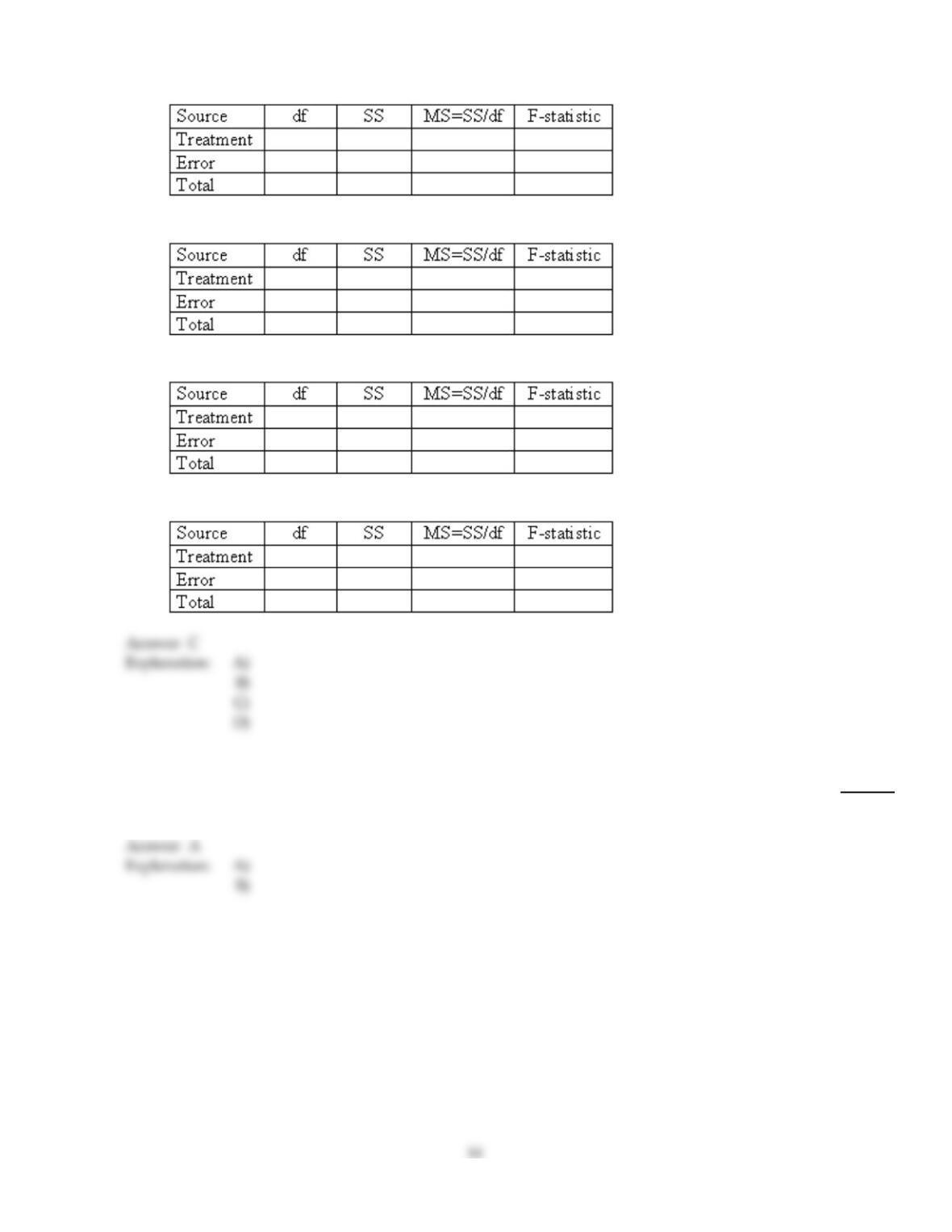
A)
388.53 29.51 0.95
12 377.47 31.46
15 466.00 31.07
B)
488.53 22.13 0.70
12 377.47 31.46
16 466.00
C)
388.53 29.51 0.94
12 377.47 31.46
15 466.00
D)
398.53 32.84 1.07
12 367.47 30.62
15 466.00
Provide an appropriate response.
37)
True or false: When performing a one–way ANOVA, the error sum of squares can be obtained by
subtracting the treatment sum of squares from the total sum of squares.
37)
A)
True
B)
False
Determine the specified calculation.
38)
Sample 1 Sample 2 Sample 3
7 2 5
6 4 5
7 3
6
MSE
38)
A)
5.667
B)
18.333
C)
9.167
D)
0.944
39)
Sample 1 Sample 2 Sample 3
8 2 5
5 4 4
9 3
6
F
39)
A)
0.521
B)
0.174
C)
5.763
D)
1.921
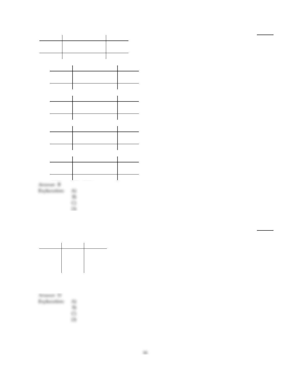
Fill in the missing entries in the partially completed one–way ANOVA table.
40)
Source df SS MS = SS/df F–statistic
Treatment 28.7
Error 25 4.2
Total 29
40)
A)
Source df SS MS = SS/df F–statistic
Treatment 428.7 0.27 0.064
Error 25 105.0 4.2
Total 29 133.7
B)
Source df SS MS = SS/df F–statistic
Treatment 4 28.7 7.18 1.71
Error 25 105.0 4.2
Total 29 133.7
C)
Source df SS MS = SS/df F–statistic
Treatment 4 28.7 7.18 1.71
Error 25 105.0 4.2
Total 29 76.3
D)
Source df SS MS = SS/df F–statistic
Treatment 4 28.7 7.18 0.59
Error 25 105.0 4.2
Total 29 133.7
Compute the sum of squares.
41)
A one–way ANOVA is to be performed. Independent random samples are selected from three
different populations. The sample data are given in the table below.
Sample 1 Sample 2 Sample 3
3 8 6
4 3 9
5 3
4
Compute the total sum of squares, SST.
41)
A)
1800
B)
240.0
C)
265.0
D)
40.0
Fill in the missing entries in the partially completed one–way ANOVA table.
42)
Source df SS MS = SS/df F–statistic
Treatment 21.1
Error 26 3.3
Total 30
42)
A)
Source df SS MS = SS/df F–statistic
Treatment 421.1 5.28 0.63
Error 26 85.8 3.3
Total 30 106.9
B)
Source df SS MS = SS/df F–statistic
Treatment 421.1 5.28 1.60
Error 26 85.8 3.3
Total 30 106.9
C)
Source df SS MS = SS/df F–statistic
Treatment 421.1 5.28 1.60
Error 26 85.8 3.3
Total 30 64.70
D)
Source df SS MS = SS/df F–statistic
Treatment 421.1 5.28 1.60
Error 26 0.13 3.3
Total 30 21.23
43)
Source df SS MS = SS/df F–statistic
Treatment 22
Error 22 3
Total 26
43)
A)
Source df SS MS = SS/df F–statistic
Treatment 422 5.50 1.83
Error 22 66.0 3
Total 26 44
B)
Source df SS MS = SS/df F–statistic
Treatment 48 22 10.33
Error 22 66.0 3
Total 26 88.0
C)
Source df SS MS = SS/df F–statistic
Treatment 422 5.50 1.83
Error 22 66.0 3
Total 26 88.0
D)
Source df SS MS = SS/df F–statistic
Treatment 422 0.33 0.11
Error 22 66.0 3
Total 26 88.0
Provide an appropriate response.
44)
A one–way ANOVA is performed to compare the means of three populations. The sample sizes are
10, 12, and 14. Determine the degrees of freedom for the F–statistic.
44)
A)
(33, 35)
B)
(2, 35)
C)
(3, 33)
D)
(2, 33)
Determine the specified calculation.
45)
Sample 1 Sample 2 Sample 3
4 2 5
5 4 5
9 2
6
SSE
45)
A)
7
B)
3.667
C)
22
D)
14
D)
Fill in the missing entries in the partially completed one–way ANOVA table.
46)
Source df SS MS = SS/df F–statistic
Treatment 21.1
Error 22 3.3
Total 26
46)
A)
Source df SS MS = SS/df F–statistic
Treatment 421.1 5.28 1.60
Error 22 72.6 3.3
Total 26 51.5
B)
Source df SS MS = SS/df F–statistic
Treatment 421.1 5.28 0.63
Error 22 72.6 3.3
Total 26 93.7
C)
Source df SS MS = SS/df F–statistic
Treatment 48 21.1 5.28 306.91
Error 22 0.15 3.3
Total 26 21.25
D)
Source df SS MS = SS/df F–statistic
Treatment 421.1 5.28 1.60
Error 22 72.6 3.3
Total 26 93.7
D)
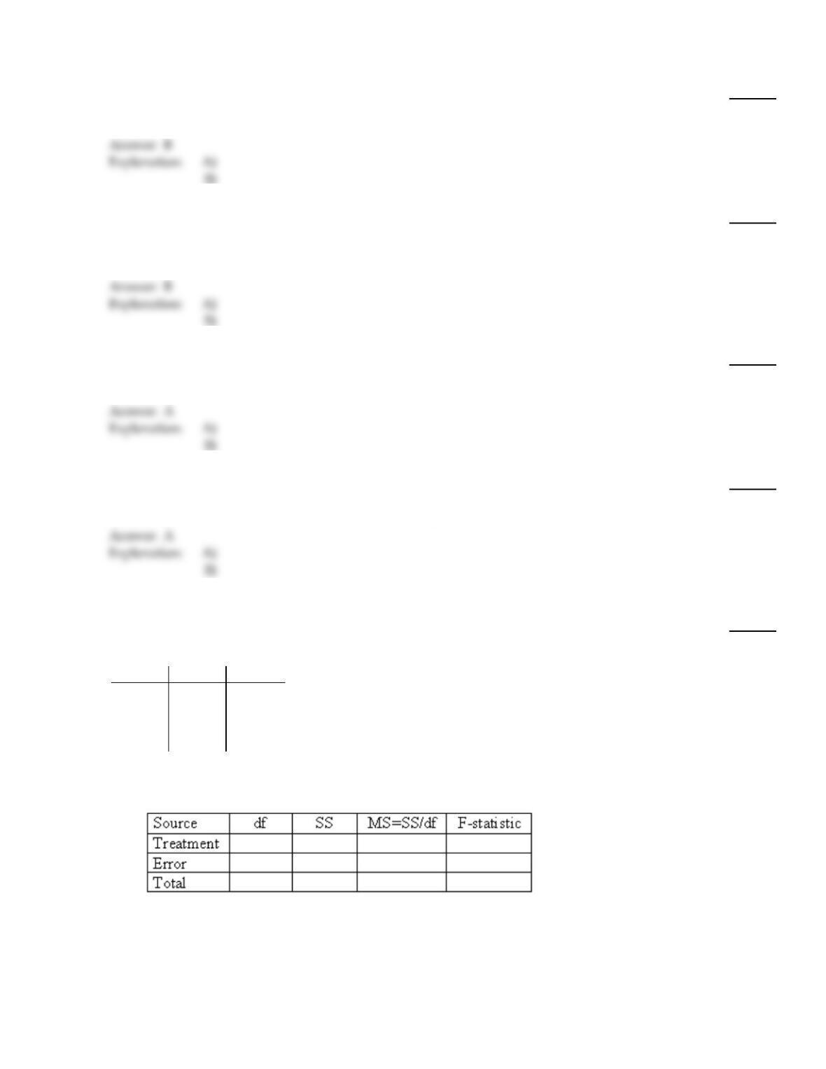
Provide an appropriate response.
47)
True or false: A one–way ANOVA test can be right–tailed, left–tailed, or two–tailed depending on
the alternative hypothesis.
47)
A)
True
B)
False
48)
A one–way ANOVA is to be performed. True or false: The error mean square gives a measure of
the variation within the samples, while the treatment mean square gives a measure of variation
among the sample means.
48)
A)
False
B)
True
49)
True or false: An F–curve is symmetrical about 0 and extends indefinitely in both directions,
approaching, but never touching, the horizontal axis as it does so.
49)
A)
False
B)
True
50)
True or false: In a one–way ANOVA, the null hypothesis will be rejected if the variation among the
sample means is large relative to the variation within the samples.
50)
A)
True
B)
False
Construct the one–way ANOVA table.
51)
A one–way ANOVA is to be performed. Independent random samples are selected from three
different populations. The sample data are given in the table below.
Sample 1 Sample 2 Sample 3
4 6 7
6 5 9
6 3 6
8 4 8
Construct the one–way ANOVA table for the data.
51)
A)
218.00 9.00 2.75
918.00 2.00
11 36.00 3.27
20
B)
318.00 6.00 3.00
918.00 2.00
12 36.00
C)
216.00 8.00 1.80
920.00 2.22
11 36.00
D)
218.00 9.00 4.50
918.00 2.00
11 36.00
Determine the specified calculation.
52)
Sample 1 Sample 2 Sample 3
8 2 5
5 4 4
6 2
5
SSTR
52)
A)
2.111
B)
7.778
C)
12.667
D)
15.556
Compute the sum of squares.
53)
A one–way ANOVA is to be performed. Independent random samples are selected from four
different populations. The sample data are given in the table below.
Sample 1 Sample 2 Sample 3 Sample 4
2 5 3 6
1 5 5 7
1 1 8
8 8
7
Compute the error sum of squares, SSE.
53)
A)
36.2
B)
67.0
C)
86.2
D)
30.8
Find the required F–value.
54)
For an F–curve with df = (24, 30), find F0.01 .
54)
A)
2.47
B)
1.67
C)
1.64
D)
2.58
Provide an appropriate response.
55)
A one–way ANOVA is performed to compare the means of four populations. The sample sizes are
24, 15, 16, and 15. Determine the degrees of freedom for the F–statistic.
55)
A)
(3, 69)
B)
(4, 66)
C)
(3, 66)
D)
(66, 69)
Determine the specified calculation.
56)
Sample 1 Sample 2 Sample 3 Sample 4 Sample 5
510 910 8
813 9 9 12
612 911
11 8 9
9
SSE
56)
A)
2.051
B)
26.667
C)
43.333
D)
10.833
Find the required F–value.
57)
For an F–curve with df = (12, 15), find F0.10 .
57)
A)
2.02
B)
3.67
C)
4.01
D)
2.10
Provide an appropriate response.
58)
True or false: In a one–way ANOVA, if the null hypothesis is rejected, we conclude that the
population means are all different (i.e., no two of the population means are equal).
58)
A)
True
B)
False
Find the required F–value.
59)
For an F–curve with df = (15, 60), find F0.005 .
59)
A)
2.57
B)
3.48
C)
1.84
D)
2.16
Fill in the missing entries in the partially completed one–way ANOVA table.
60)
Source df SS MS = SS/df F–statistic
Treatment 322.97 11.16
Error 13.72 0.686
Total
60)
A)
Source df SS MS = SS/df F–statistic
Treatment 322.97 7.66 11.16
Error 20 13.72 0.686
Total 23 36.69
B)
Source df SS MS = SS/df F–statistic
Treatment 322.97 1.15 1.68
Error 20 13.72 0.686
Total 23 36.69
C)
Source df SS MS = SS/df F–statistic
Treatment 322.97 1.67 2.43
Error 20 13.72 0.686
Total 23 36.69
D)
Source df SS MS = SS/df F–statistic
Treatment 322.97 7.66 11.16
Error 20 13.72 0.686
Total 23 9.25
61)
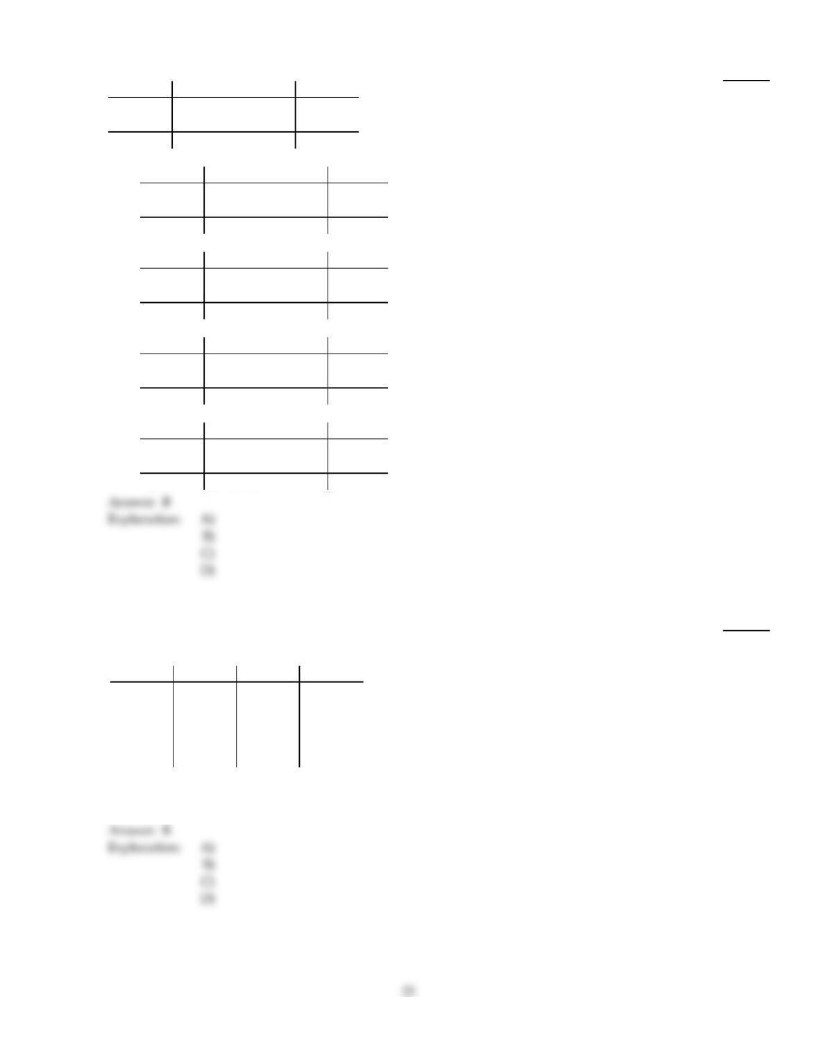
Source df SS MS = SS/df F–statistic
Treatment 20.5
Error 29 3.9
Total 34
61)
A)
Source df SS MS = SS/df F–statistic
Treatment 5 20.5 4.10 0.95
Error 29 113.1 3.9
Total 34 133.6
B)
Source df SS MS = SS/df F–statistic
Treatment 520.5 4.10 1.05
Error 29 113.1 3.9
Total 34 133.6
C)
Source df SS MS = SS/df F–statistic
Treatment 520.5 4.10 1.05
Error 29 113.1 3.9
Total 34 92.6
D)
Source df SS MS = SS/df F–statistic
Treatment 520.5 0.18 0.046
Error 29 113.1 3.9
Total 34 133.6
Compute the sum of squares.
62)
A one–way ANOVA is to be performed. Independent random samples are selected from four
different populations. The sample data are given in the table below.
Sample 1 Sample 2 Sample 3 Sample 4
5 8 3 6
3 7 5 3
8 1 5
8 1
7
Compute the treatment sum of squares, SSTR.
62)
A)
80.0
B)
19.3
C)
136.5
D)
369.3
Find the required F–value.
63)
For an F–curve with df = (20, 5), find F0.025 .
63)
A)
6.33
B)
4.10
C)
3.29
D)
4.56
64)
An F–curve has df = (15, 24). Find the F–value having area 0.025 to its right.
64)
A)
2.11
B)
2.44
C)
3.29
D)
2.70
65)
An F–curve has df = (8, 15). Find the F–value having area 0.05 to its right.
65)
A)
2.64
B)
3.22
C)
4.67
D)
6.81
66)
For an F–curve with df = (60, 10), find F0.05 .
66)
A)
2.90
B)
1.99
C)
2.62
D)
4.86
Fill in the missing entries in the partially completed one–way ANOVA table.
67)
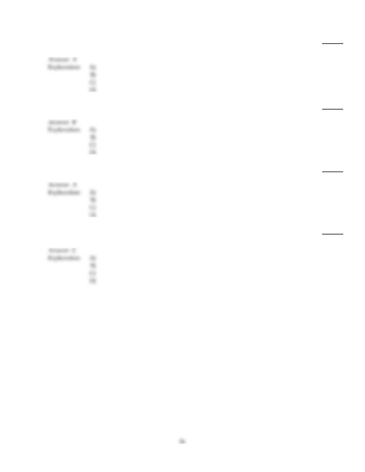
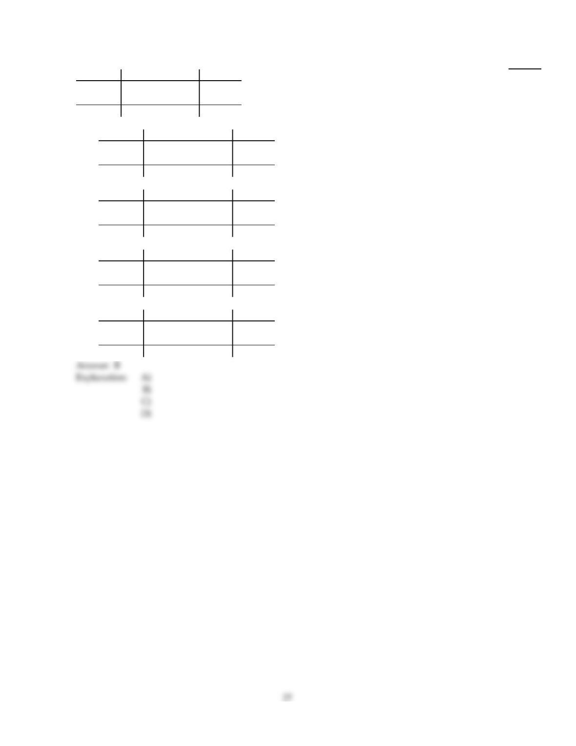
Source df SS MS = SS/df F–statistic
Treatment 24
Error 29 4.8
Total 33
67)
A)
Source df SS MS = SS/df F–statistic
Treatment 424 6.00 0.80
Error 29 139.2 4.8
Total 33 163.2
B)
Source df SS MS = SS/df F–statistic
Treatment 424 6.00 1.25
Error 29 139.2 4.8
Total 33 163.2
C)
Source df SS MS = SS/df F–statistic
Treatment 62 24 0.39 0.08
Error 29 139.2 4.8
Total 33 163.2
D)
Source df SS MS = SS/df F–statistic
Treatment 424 6.00 1.25
Error 29 139.2 4.8
Total 33 5.8
68)
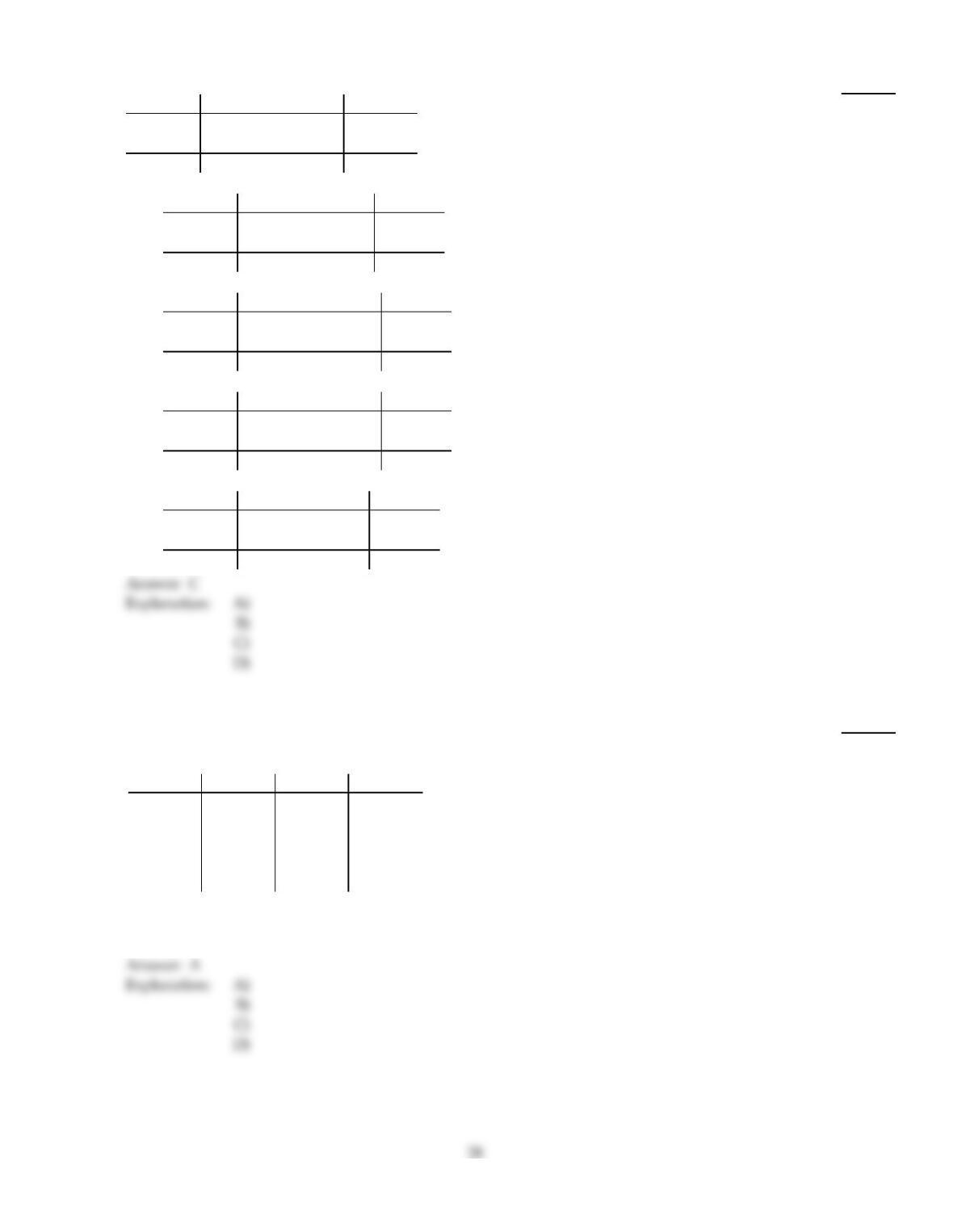
Source df SS MS = SS/df F–statistic
Treatment 22.2
Error 23 4
Total 27
68)
A)
Source df SS MS = SS/df F–statistic
Treatment 50 22.2 0.44 0.111
Error 23 92.0 4
Total 27 70.0
B)
Source df SS MS = SS/df F–statistic
Treatment 422.2 0.44 9.09
Error 23 92.0 4
Total 27 114.2
C)
Source df SS MS = SS/df F–statistic
Treatment 422.2 5.55 1.39
Error 23 92.0 4
Total 27 114.2
D)
Source df SS MS = SS/df F–statistic
Treatment 422.2 5.55 1.39
Error 23 92.0 4
Total 27 69.8
Compute the sum of squares.
69)
A one–way ANOVA is to be performed. Independent random samples are selected from four
different populations. The sample data are given in the table below.
Sample 1 Sample 2 Sample 3 Sample 4
2 5 3 4
3 4 5 9
2 1 9
8 8
7
Compute the total sum of squares, SST.
69)
A)
98.0
B)
153.0
C)
128.0
D)
4550
Determine the specified calculation.
70)
Sample 1 Sample 2 Sample 3 Sample 4 Sample 5
610 810 8
913 8 9 12
11 12 911
11 8 9
9
MSE
70)
A)
2.667
B)
19.611
C)
34.667
D)
4.903
Compute the sum of squares.
71)
A one–way ANOVA is to be performed. Independent random samples are selected from three
different populations. The sample data are given in the table below.
Sample 1 Sample 2 Sample 3
3 5 6
3 4 9
3 8
7
Compute the error sum of squares, SSE.
71)
A)
67.5
B)
5.5
C)
73.0
D)
230.5
Determine the specified calculation.
72)
Sample 1 Sample 2 Sample 3 Sample 4 Sample 5
310 410 8
10 13 8 9 12
12 12 911
11 8 9
9
MSTR
72)
A)
41.333
B)
74.667
C)
5.744
D)
10.333
73)
Sample 1 Sample 2 Sample 3 Sample 4 Sample 5
410 12 10 8
913 11 912
612 911
11 8 9
9
F
73)
A)
0.212
B)
0.688
C)
1.453
D)
4.724
Fill in the missing entries in the partially completed one–way ANOVA table.
74)
Source df SS MS = SS/df F–statistic
Treatment 24.1
Error 30 3.2
Total 34
74)
A)
Source df SS MS = SS/df F–statistic
Treatment 424.1 6.03 1.88
Error 30 96.0 3.2
Total 34 120.1
B)
Source df SS MS = SS/df F–statistic
Treatment 424.1 6.03 0.53
Error 30 96.0 3.2
Total 34 120.1
C)
Source df SS MS = SS/df F–statistic
Treatment 424.1 0.38 482.00
Error 30 96.0 3.2
Total 34 120.1
D)
Source df SS MS = SS/df F–statistic
Treatment 424.1 6.03 1.88
Error 30 96.0 3.2
Total 34 24.21
Determine the specified calculation.
75)
Sample 1 Sample 2 Sample 3 Sample 4 Sample 5
510 13 10 8
813 11 912
12 12 911
11 8 9
9
SSTR
75)
A)
3.744
B)
25.333
C)
48.667
D)
6.333
Answer Key
Testname: C13
32
Answer Key
Testname: C13
33
Answer Key
Testname: C13
Answer Key
Testname: C13