
Name:
Class:
Date:
chapter 12
Indicate whether the statement is true or false.
1. To deseasonalize an observation (assuming a multiplicative model of seasonality), multiply it by the appropriate
seasonal index.
a.
True
b.
False
2. We compute the five-period moving averages for all time periods except the first two.
a.
True
b.
False
3. The purpose of using the moving average is to take away the short-term seasonal and random variation, leaving behind
a combined trend and cyclical movement.
a.
True
b.
False
4. Econometric forecasting models, also called causal models, use regression to forecast a time series variable by using
other explanatory time series variables.
a.
True
b.
False
5. Correlogram is a bar chart of autocorrelation at different lags.
a.
True
b.
False
6. If the observations of a time series increase or decrease regularly through time, we say that the time series has a
random (or noise) component.
a.
True
b.
False
7. If a time series exhibits an exponential trend, then a plot of its logarithm should be approximately linear.
a.
True
b.
False
8. The time series component that reflects a long-term, relatively smooth pattern or direction exhibited by a time series
over a long time period, is called seasonal.
a.
True
b.
False
9. A time series can consist of four different components: trend, seasonal, cyclical, and random (or noise).
a.
True
b.
False
10. A shortcoming of the RMSE (root mean square error) is that it is not in the same units as the forecast variable.
a.
True
b.
False
11. Forecasting software packages typically report several summary measures of the forecasting error. The most

Name:
Class:
Date:
chapter 12
important of these are MAE (mean absolute error), RMSE (root mean square error), and MAPE (mean absolute
percentage error).
a.
True
b.
False
12. The null hypothesis in a runs test is the data series is random
a.
True
b.
False
13. Simple exponential smoothing is appropriate for a series without a pronounced trend or seasonality.
a.
True
b.
False
14. The smoothing constant used in simple exponential smoothing is analogous to the span in moving averages.
a.
True
b.
False
15. An autocorrelation is a type of correlation used to measure whether the values of a time series are related to their own
past values.
a.
True
b.
False
16. If we use a value close to 1 for the smoothing constant in a simple exponential smoothing model, then we expect the
model to respond very slowly to changes in the level.
a.
True
b.
False
17. The runs test is a formal test of the null hypothesis of randomness. If there are too many or too few runs in the series,
then we conclude that the series is not random.
a.
True
b.
False
18. The seasonal component of a time series is more likely to exhibit the relatively steady growth of a variable, such as
the population of Egypt from 35 million in 1960 to 75 million in 2005.
a.
True
b.
False
19. Holt’s method is an exponential smoothing method, which is appropriate for a series with seasonality and possibly a
trend.
a.
True
b.
False
20. In an additive seasonal model, we add an appropriate seasonal index to a “base” forecast. These indexes, one for
each season, typically average to 0.
a.
True
b.
False
21. You will always get more accurate forecasts by using more complex forecasting methods.

Name:
Class:
Date:
chapter 12
a.
True
b.
False
22. The most common form of autocorrelation is positive autocorrelation, where large observations tend to follow large
observations and small observations tend to follow small observations.
a.
True
b.
False
23. A moving average is the average of the observations in the past few periods, where the number of terms in the
average is the span.
a.
True
b.
False
24. Winter’s method is an exponential smoothing method, which is appropriate for a series with trend but no seasonality.
a.
True
b.
False
25. In a random walk model, there are significantly more runs than expected, and the autocorrelations are not significant.
a.
True
b.
False
26. A trend component of a time series is a long-term, relatively smooth pattern or direction exhibited by a series, and its
duration is more than one year.
a.
True
b.
False
27. A meandering pattern is an example of a random time series.
a.
True
b.
False
28. In a regression model with seasonal dummy variables, the coefficients on the dummy variables represent the additive
factor relative to the reference quarter value, not the multiplicative factor.
a.
True
b.
False
29. The seasonal component of a time series is harder to predict than the cyclic component; the reason is that cyclic
variation is much more regular.
a.
True
b.
False
30. Seasonal variations will not be present in a deseasonalized time series.
a.
True
b.
False
31. As is the case with residuals from regression, the forecast errors for nonregression methods will always average to
zero
a.
True
Name:
Class:
Date:
chapter 12
b.
False
32. The moving average method is perhaps the simplest and one of the most frequently-used extrapolation methods.
a.
True
b.
False
33. Extrapolation forecasting methods are quantitative methods that use past data of a time series variable – and nothing
else, except possible time itself – to forecast values of the variable.
a.
True
b.
False
34. If the span of a moving average is large – say, 12 months – then few observations go into each average, and extreme
values have relatively large effect on the forecasts.
a.
True
b.
False
35. In a multiplicative seasonal model, we multiply a “base” forecast by an appropriate seasonal index. These indexes,
one for each season, typically average to 1.
a.
True
b.
False
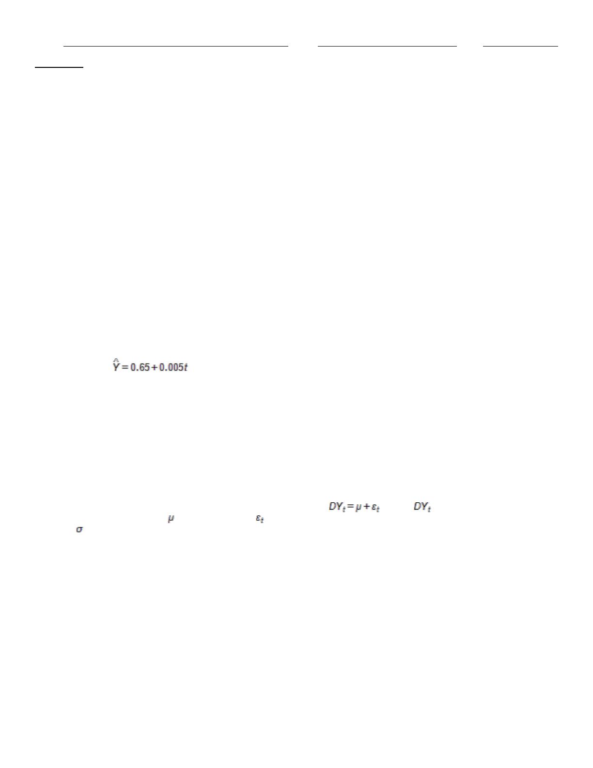
36. The trend line was calculated from quarterly data for 2000 – 2004, where t = 1 for the first quarter of
2000. The trend value for the second quarter of the year 2005 is 0.75.
a.
True
b.
False
37. The time series component that reflects a wavelike pattern describing a long-term trend that is generally apparent over
a number of years is called cyclical.
a.
True
b.
False
38. An equation for the random walk model is given by the equation: , where is the change in the time
series from time t to time t – 1, is a constant, and is a random variable (noise) with mean 0 and some standard
deviation .
a.
True
b.
False
39. In exponential smoothing models, the forecast is based on the level at time t, Lt, which is not observable and can only
be estimated.
a.
True
b.
False
40. The cyclic component of a time series is more likely to exhibit business cycles that record periods of economic
recession and inflation.
a.
True
b.
False

Name:
Class:
Date:
chapter 12
41. An exponential trend is appropriate when the time series changes by a constant percentage each period.
a.
True
b.
False
42. To calculate the five-period moving average for a time series, we average the values in the two preceding periods,
and the values in the three following time periods.
a.
True
b.
False
43. The smoothing constants in exponential smoothing models are effectively a way to assign different weights to past
levels, trends and cycles in the data.
a.
True
b.
False
44. Regression models with seasonal dummy variables produce coefficients for each quarter, which represent the additive
or multiplicative factors relative to the annual average.
a.
True
b.
False
45. If a random series has too few runs, then it is zigzagging too often.
a.
True
b.
False
46. Every form of exponential smoothing model has at least one smoothing constant, which is always between 0 and 1.
a.
True
b.
False
47. If we use a value close to 1 for the level smoothing constant and a value close to 0 for the trend smoothing constant
in Holt’s exponential smoothing model, then we expect the model to respond very quickly to changes in the level, but
very slowly to changes in the trend.
a.
True
b.
False
48. We compare the percent of variation explained R2 for a regression model with seasonal dummy variables to the
MAPE for the smoothing model with seasonality to see which model is more accurate.
a.
True
b.
False
49. A time series is any variable that is measured over time in sequential order.
a.
True
b.
False
Indicate the answer choice that best completes the statement or answers the question.
50. Which of the following summary measures for forecast errors does not depend on the units of the forecast variable?
a.
MAE (mean absolute error)
b.
MFE (mean forecast error)

Name:
Class:
Date:
chapter 12
c.
RMSE (root mean square error)
d.
MAPE (mean absolute percentage error)
51. Econometric models can also be called:
a.
judgmental models
b.
time series models
c.
causal models
d.
environmetric models
52. Suppose that a simple exponential smoothing model is used (with a = 0.30) to forecast monthly sandwich sales at a
local sandwich shop. After June’s demand is observed at 1520 sandwiches, the forecasted demand for July is 1600
sandwiches. At the beginning of July, what would be the forecasted demand for August?
a.
1520
b.
1544
c.
1550
d.
1600
53. There are a variety of deseasonalizing methods, but they are typically variations of:
a.
ratio-to-seasonality methods
b.
ratio-to-exponential-smoothing methods
c.
ratio-to-moving-average methods
d.
linear trend
54. Extrapolation methods attempt to:
a.
use non-quantitative methods to predict future values
b.
search for patterns in the data and then use those to predict future values
c.
find variables that are correlated with the data being predicted
d.
predict the next period’s value by using the latest period’s value
55. The most common form of autocorrelation is positive autocorrelation, in which:
a.
large observations tend to follow both large and small observations
b.
small observations tend to follow both large and small observations
c.
large observations tend to follow large observations and small observations tend to follow small observations
d.
large observations tend to follow small observations and small observations tend to follow large observations
56. When using Holt’s model, choosing values of the smoothing constant that are near 1 will result in forecast models
which
a.
react very quickly to changes in the level
b.
react very quickly to changes in the trend
c.
react very quickly to changes in the level and the trend
d.
react very slowly to changes in the level and the trend
57. The linear trend was estimated using a time series with 20 time periods. The forecasted value for time
period 21 is
a.
120
Name:
Class:
Date:
chapter 12
b.
122
c.
160
d.
162
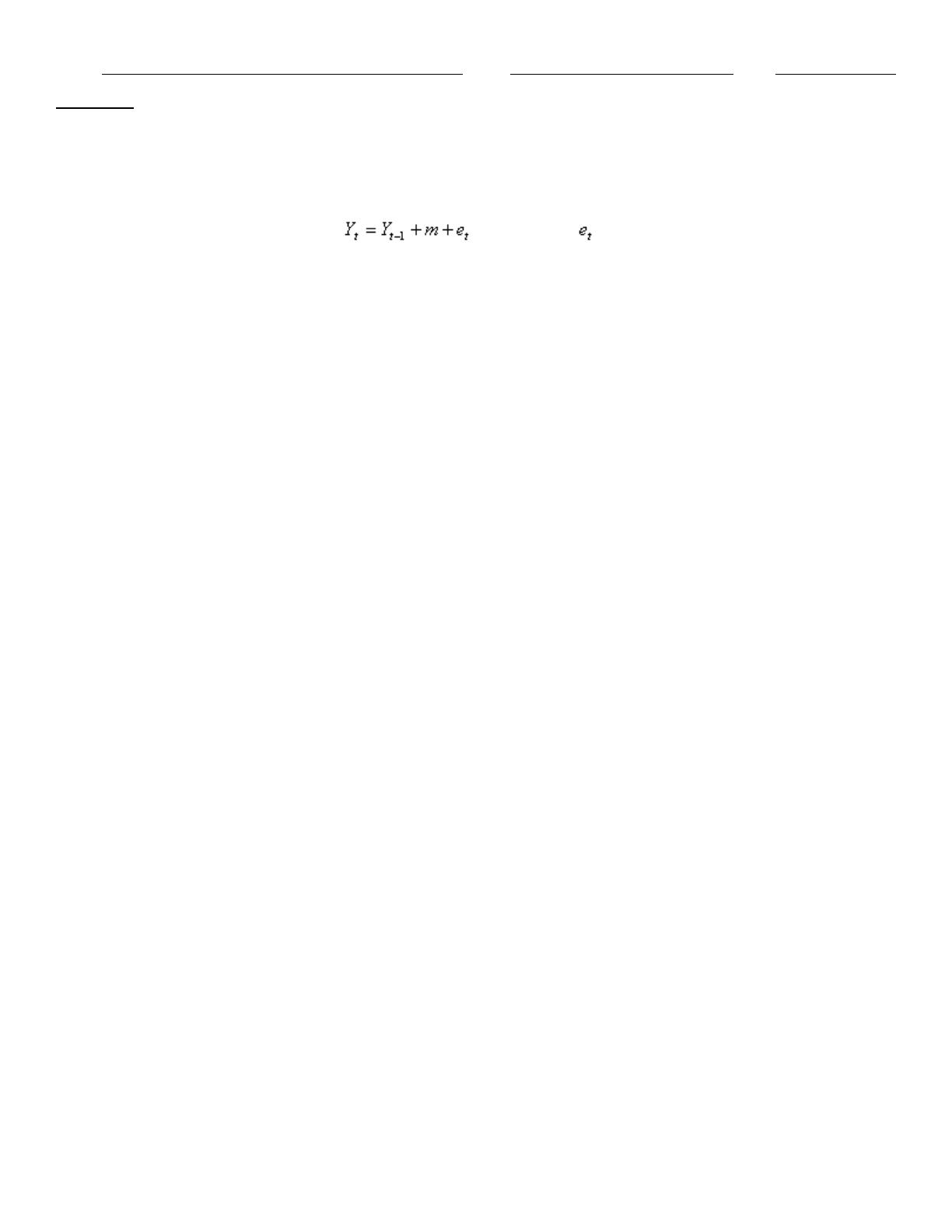
58. The random walk model is written as: . In this model, represents the:
a.
average of the Y’s
b.
average of the X’s
c.
forecasted value
d.
random series with mean 0 and some constant standard deviation
59. The components of a time series include:
a.
base series
b.
trend
c.
seasonal component
d.
cyclic component
e.
all of these options
60. Which of the following is not a method for dealing with seasonality in data
a.
Winter’s exponential smoothing model
b.
deseasonalizing the data, using any forecasting model, then reseasonalizing the data
c.
multiple regression with lags for the seasons
d.
multiple regression with dummy variables for the seasons
61. When using the moving average method, you must select which represent(s) the number of terms in the moving
average.
a.
a smoothing constant
b.
the explanatory variables
c.
an alpha value
d.
a span
62. Examples of non-random patterns that may be evident on a time series graph include:
a.
trends
b.
increasing variance over time
c.
a meandering pattern
d.
too many zigzags
e.
all of these options
63. Holt’s model differs from simple exponential smoothing in that it includes a term for:
a.
seasonality
b.
trend
c.
residuals
d.
cyclical fluctuations
64. Models such as moving average, exponential smoothing, and linear trend use only:
a.
future values of Y to forecast previous values of Y
Name:
Class:
Date:
chapter 12
b.
previous values of Y to forecast future values of Y
c.
multiple explanatory variables (not just values of Y) to forecast future values of Y
d.
ratio-to-moving-average methods
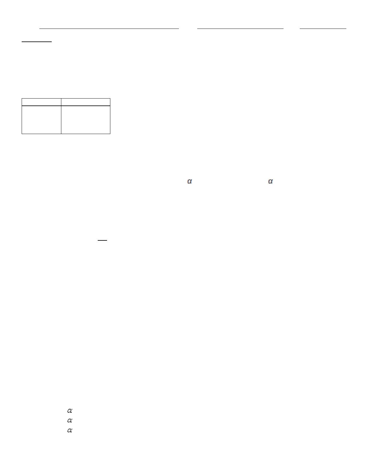
65. The data below represents sales for a particular product. If you were to use the moving average method with a span of
3 periods, what would be your forecast for period 5?
Period
Sales (in units)
1
90
2
120
3
110
4
100
a.
90
b.
100
c.
105
d.
110
66. When using exponential smoothing, a smoothing constant must be used. The value for :
a.
ranges between 0 and 1
b.
ranges between –1 and +1
c.
equals the largest observed value in the series
d.
represents the strength of the association between the forecasted and observed values
67. Which of the following is not one of the techniques that can be used to identify whether a time series is truly random?
a.
A graph (plot the data)
b.
The runs test
c.
A control chart
d.
The autocorrelations (or a correlogram)
68. In contrast to linear trend, exponential trend is appropriate when the time series changes by a:
a.
constant amount each time period
b.
constant percentage each time period
c.
positive amount each time period
d.
negative amount each time period
69. Winters’ model differs from Holt’s model and simple exponential smoothing in that it includes an index for:
a.
seasonality
b.
trend
c.
residuals
d.
cyclical fluctuations
70. When using exponential smoothing, if you want the forecast to react quickly to movements in the series, you should
choose:
a.
values of near 1
b.
values of near 0
c.
values of midway between 0 and 1
d.
it depends on the data set

Name:
Class:
Date:
chapter 12
71. Perhaps the simplest and one of the most frequently used extrapolation methods is the:
a.
moving average
b.
linear trend
c.
exponential trend
d.
causal model
72. The following are the values of a time series for the first four time periods:
t
1
2
3
4
24
25
26
27
Using a four-period moving average, the forecasted value for time period 5 is:
a.
24.5
b.
25.5
c.
26.5
d.
27.5
73. Related to the runs test, if T is reasonably large (T > 20 is suggested), then the statistic can be used to perform this
test.
a.
F
b.
t
c.
Z
d.
74. In a random walk model the
a.
series itself is random
b.
series itself is not random but its differences are random
c.
series itself and its differences are random
d.
series itself and its differences are not random
75. Related to the runs test, if you use a Z-statistic and you get a Z value greater than 2.0, this means that there is
evidence of _____in the series
a.
randomness
b.
nonrandomness
c.
nonnormality
d.
heteroscedasticity
76. The idea behind the runs test is that a random number series should have a number of runs that is:
a.
large
b.
small
c.
not large or small
d.
constant
77. In a random series, successive observations are probabilistically independent of one another. If this property is
violated, the observations are said to be:
a.
autocorrelated

Name:
Class:
Date:
chapter 12
b.
intercorrelated
c.
causal
d.
seasonal
78. The moving average method can also be referred to as a (n) method.
a.
causal
b.
smoothing
c.
exponential
d.
econometric
79. A linear trend means that the time series variable changes by a:
a.
constant amount each time period
b.
constant percentage each time period
c.
positive amount each time period
d.
negative amount each time period
80. The runs test uses a series of 0’s and 1’s. The 0’s and 1’s represent whether each observation is:
a.
above or below the predicted value of Y
b.
above or below the mean value of Y
c.
is above or below the mean value of the previous two observations
d.
is positive or negative
81. Suppose that a simple exponential smoothing model is used (with = 0.40) to forecast monthly sandwich sales at a
local sandwich shop. The forecasted demand for September was 1560 and the actual demand was 1480 sandwiches.
Given this information, what would be the forecast number of sandwiches for October?
a.
1480
b.
1528
c.
1560
d.
1592
82. A regression approach can also be used to deal with seasonality by using variables for the seasons.
a.
smoothing
b.
response
c.
residual
d.
dummy
83. The data below represents sales for a particular product. If you were to use the moving average method with a span of
4 periods, what would be your forecast for period 5?
Period
Sales (in units)
1
90
2
120
3
110
4
100
a.
90
b.
100
c.
105
Name:
Class:
Date:
chapter 12
d.
110
84. Forecasting models can be divided into three groups. They are:
a.
time series, optimization, and simulation methods
b.
judgmental, extrapolation, and econometric methods
c.
judgmental, random, and linear methods
d.
linear, non-linear, and extrapolation methods
85. The forecast error is the difference between
a.
this period’s value and the next period’s value
b.
the average value and the expected value of the response variable
c.
the explanatory variable value and the response variable value
d.
the actual value and the forecast
86. Which of the following is not one of the summary measures for forecast errors that is commonly used?
a.
MAE (mean absolute error)
b.
MFE (mean forecast error)
c.
RMSE (root mean square error)
d.
MAPE (mean absolute percentage error)
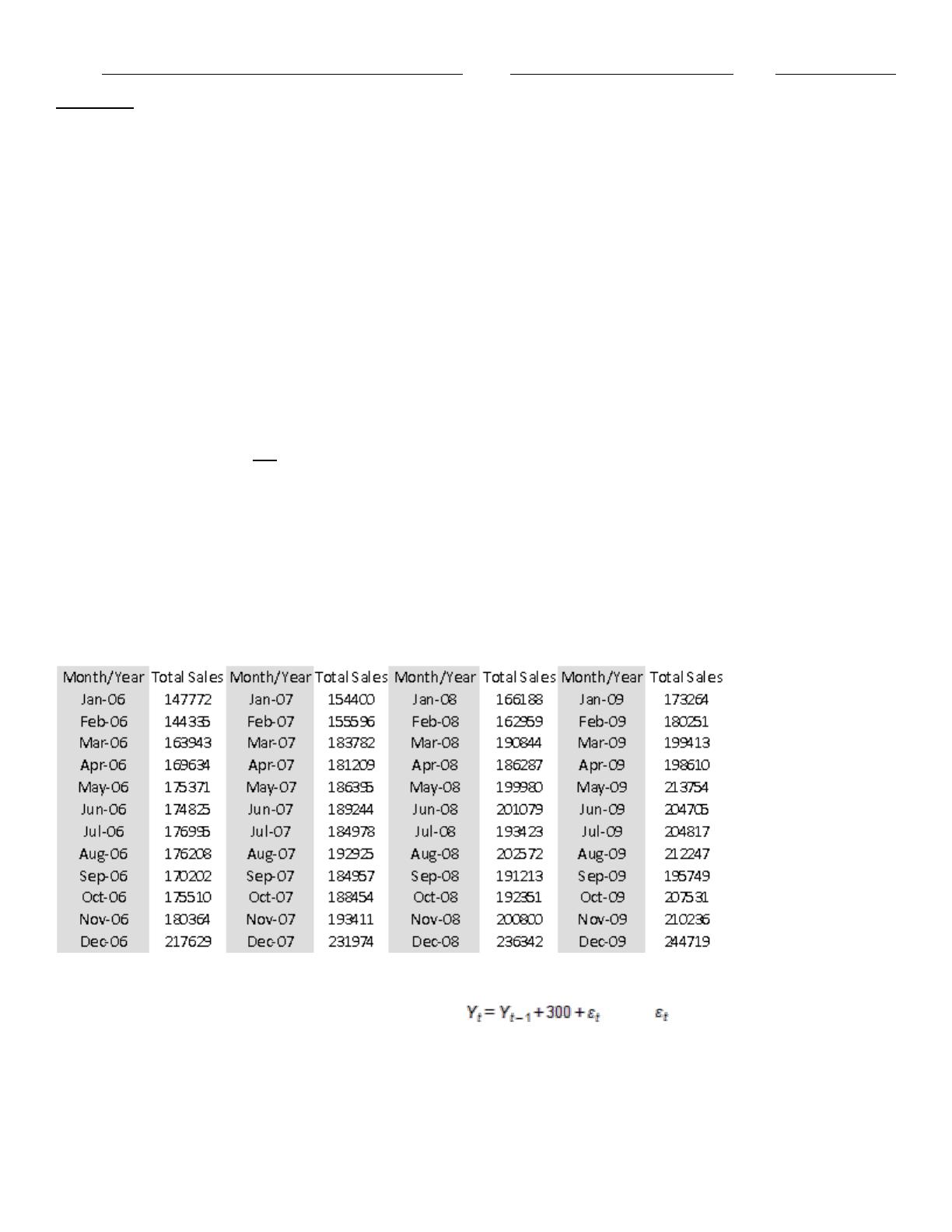
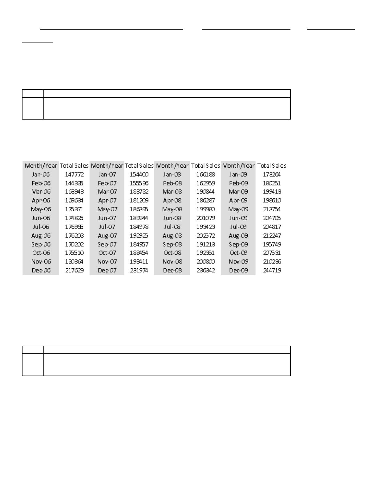
The data shown below contains total monthly retail sales (in dollars) a small sporting goods store for the years 2006–
2008.
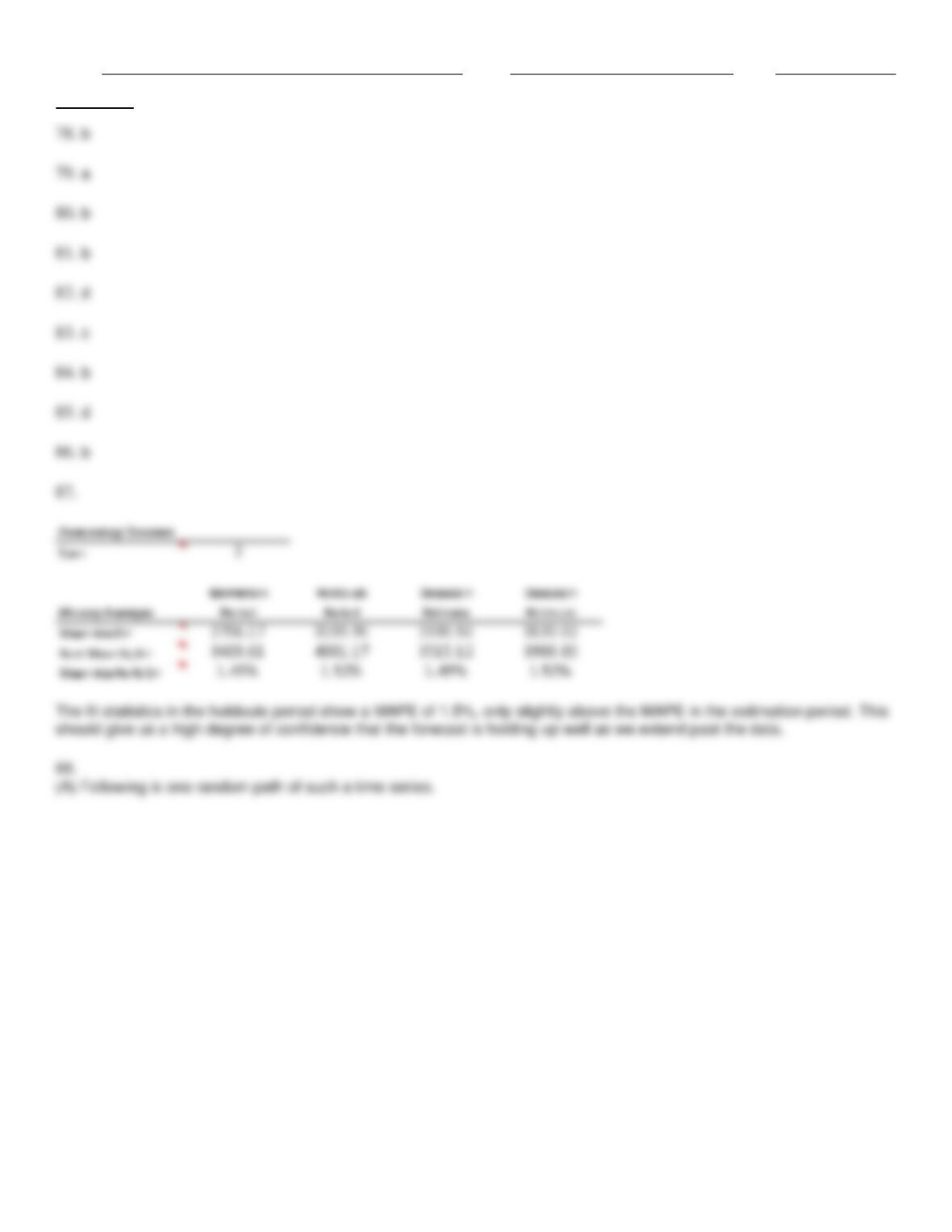
87. Run the moving average fit again, this time holding out the last 6 observations to validate the fit. What do you find?
Consider a random walk model with the following equation: , where is a normally distributed random
series with mean of 0 and standard deviation of 12.
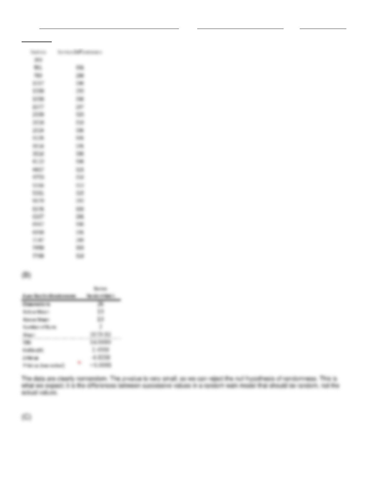
88. (A) Use Excel to generate a time series of 25 values using this random walk model with a starting value of 200.
(B) Conduct a runs test on the series you generated for (A). Is it random? Explain.
(C) Conduct a runs test on the differences between successive values for the series you generated for (A). Is it random?
Explain.
Name:
Class:
Date:
chapter 12
(D) Use the time series you constructed in (A) to forecast the next observation.
The number of employees on the payroll at a computer software company is recorded at the start of each month from
January 2007 to December 2009. These data are shown below.
Year
Jan
Feb
March
April
May
June
July
Aug.
Sept.
Oct.
Nov.
Dec
2007
348
352
330
347
339
370
380
392
400
410
405
367
2008
350
341
345
355
342
350
370
395
410
401
405
365
2009
348
349
350
350
342
377
369
400
410
406
400
370
89. Perform a runs test and compute a few autocorrelations to determine whether this time series is random.
The data shown below contains total monthly retail sales (in dollars) a small sporting goods store for the years 2006–
2008.
90. Use the method of moving averages with an appropriate span to forecast retail sales for the first half of 2009. Do you
obtain a good fit? Do you have confidence in your forecast? Explain your answers.
91. Obtain a time series graph of the data. If you will be using a moving average model of the data, what information does
this graph provide to help specify such a model?
The number of employees on the payroll at a computer software company is recorded at the start of each month from
January 2007 to December 2009. These data are shown below.
Year
Jan
Feb
March
April
May
June
July
Aug.
Sept.
Oct.
Nov.
Dec
2007
348
352
330
347
339
370
380
392
400
410
405
367
2008
350
341
345
355
342
350
370
395
410
401
405
365
2009
348
349
350
350
342
377
369
400
410
406
400
370
92. Use the method of moving averages with an appropriate span to forecast retail sales for 2010. Do you obtain a good
fit? Do you have confidence in your forecast? Explain your answers.
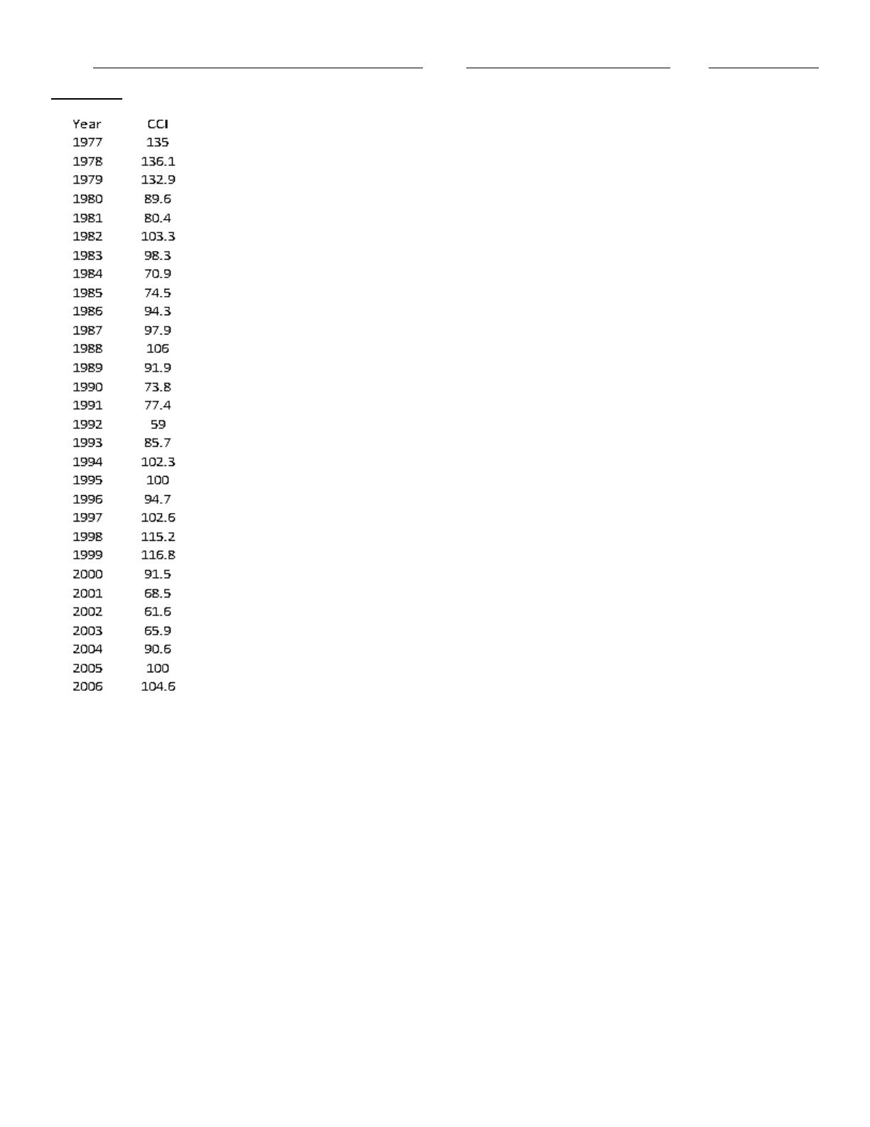
The Consumer Confidence Index (CCI) attempts to measure people’s feelings about general business conditions,
employment opportunities, and their own income prospects. The data shown below contains the annual average values of
the CCI for the period 1977–2006.
Name:
Class:
Date:
chapter 12
93. Obtain an autocorrelation table for this series.
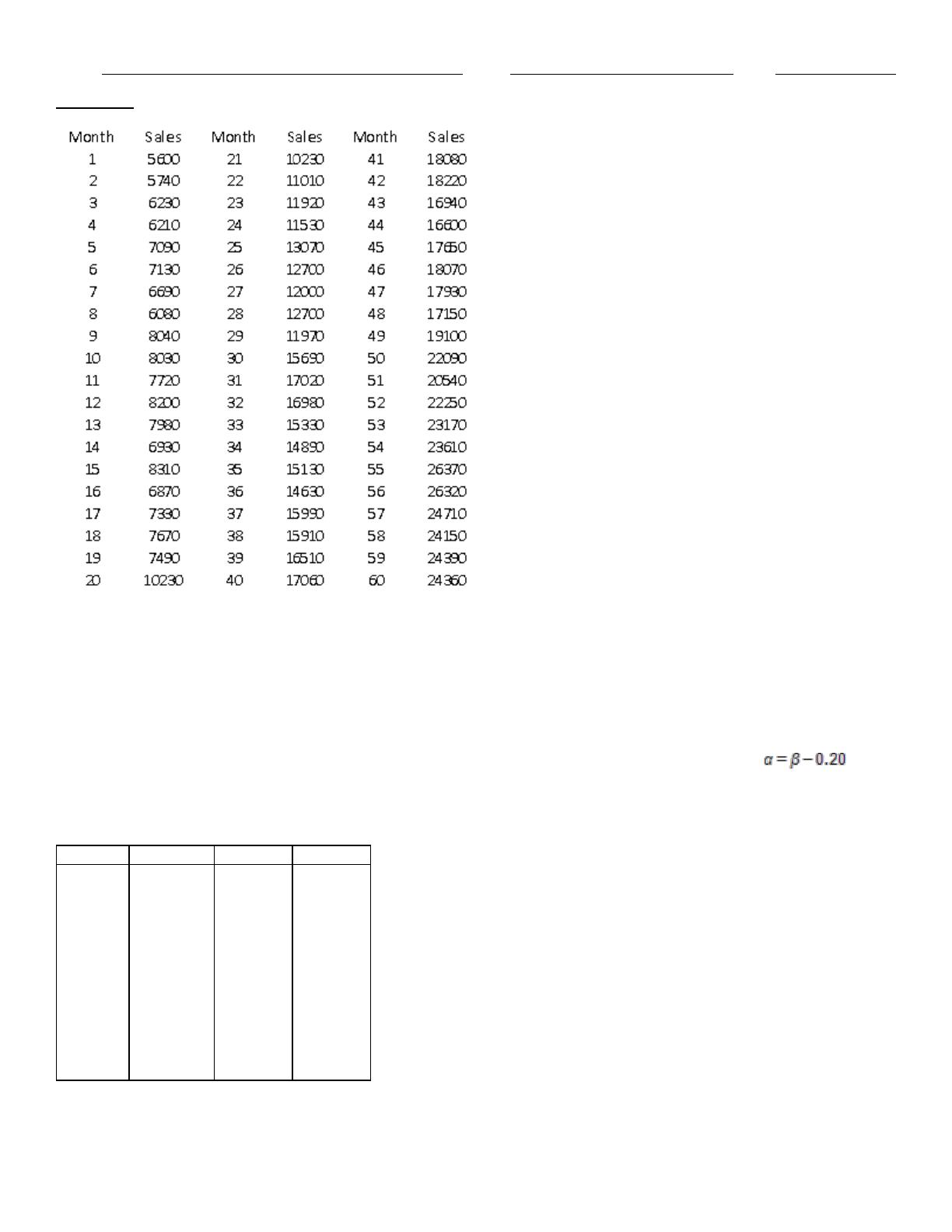
The table below contains 5 years of monthly data on sales (number of units sold) for a particular company, in
addition to extra columns containing information needed to answer some of the questions. The company
suspects that except for random noise, its sales are growing by a constant percentage each month and that they
will continue to do so for at least the near future.
Name:
Class:
Date:
chapter 12
94. (A) Fit the appropriate regression model to the data. Report the resulting equation and state explicitly what it says
about the percentage growth per month.
(B) What is the MAPE for the forecast model in (A)? What does it measure? Considering its magnitudes, does the model
seem to be doing a good job?
95. A car dealer in Big Rapids, Michigan is using Holt’s method to forecast weekly car sales. Currently the level is
estimated to be 45 cars per week, and the trend is estimated to be 5 cars per week. During the current week, 25 cars are
sold. After observing the current week’s sales, forecast the number of cars three weeks from now. Use .
The data shown below contains the monthly sales (in thousands of dollars) at a local department store for each of the past
24 months.
Month
Sales
Month
Sales
1
987
13
1080
2
1080
14
1002
3
975
15
968
4
1060
16
984
5
1030
17
1045
6
895
18
945
7
908
19
1025
8
1059
20
950
9
940
21
1004
10
1038
22
1075
11
1050
23
969
12
1030
24
1029
96. (A) Develop a time series plot of the data.
(B) Perform a runs test and compute a few autocorrelations to determine whether this time series is random.
Name:
Class:
Date:
chapter 12
(C) Given your answers to (A) and (B), what type of forecast do you recommend? Explain your answer.
(D) Use your answer to (C), to obtain a forecast for the next quarter (4 months). How reliable do you think this forecast is?
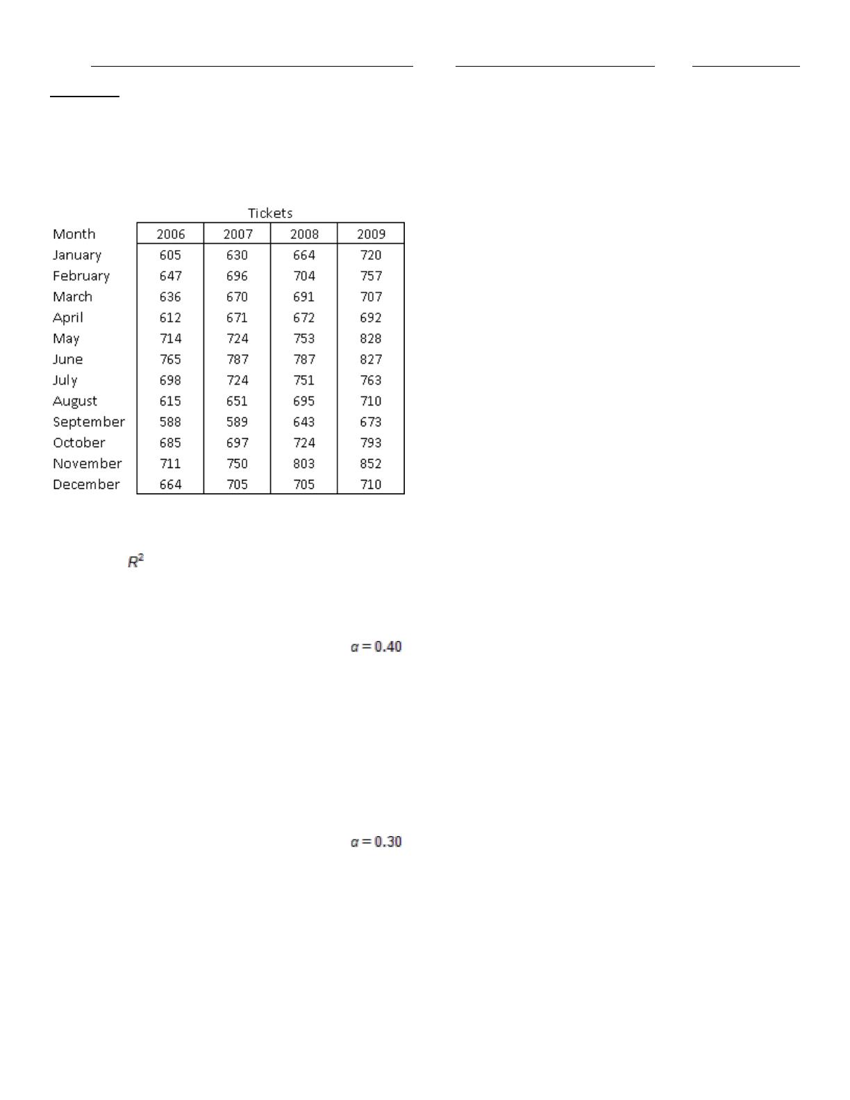
The table below contains the monthly number of airline tickets sold by a travel agency in Grand Rapids, Michigan
97. (A) Is this time series random? Perform a runs test and compute a few autocorrelations to support your answer.
(B) Does a linear trend appear to fit these data well? If so, estimate the linear-trend model for this time series, and
interpret the value.
(C) Is there evidence of some seasonal pattern in these sales data? If so, characterize the seasonal pattern, and explain
how to forecast future values.
Suppose that simple exponential smoothing with is used to forecast monthly wine sales at a liquor store. After
April’s demand is observed, the forecasted demand for May is 4500 bottles of wine.
98. (A) At the beginning of May, what is the forecast of July’s wine sales?
(B) Suppose that actual demands during May and June are as follows: May, 5000 bottle of wine; June 4000 bottle of wine.
After observing June’s demand, what is the forecast for July’s demand?
(C) Based on the data from (B), the demands during May and June average (5000+4000)/2 = 4500 bottle per month. This
is the same as the forecast for monthly sales before we observed the May and June data. Yet after we observe the May
and June demands for wine, our forecast for July demand has decreased from what it was at the end of April. Why?
Suppose that simple exponential smoothing with is used to forecast monthly Pepsi sales at a small grocery store.
After March’s demand is observed, the forecasted demand for April is 5000 cans of Pepsi.
99. (A) Suppose that actual demands during April and May are as follows: May, 5500 cans; June 4500 cans. After
observing May’s demand, what is the forecast for June’s demand?
(B) Based on the data from (A), the demands during April and May average (5500+4500)/2 = 5000 cans per month. This
is the same as the forecast for monthly sales before we observed the April and May data. Yet after we observed the April
and May demands for Pepsi, our forecast for June demand has decreased from what it was at the end of March. Why?
100. The number of reported accidents at a manufacturing plant located in Flint, Michigan, was recorded at the start of
each month. These data are provided in the table below:
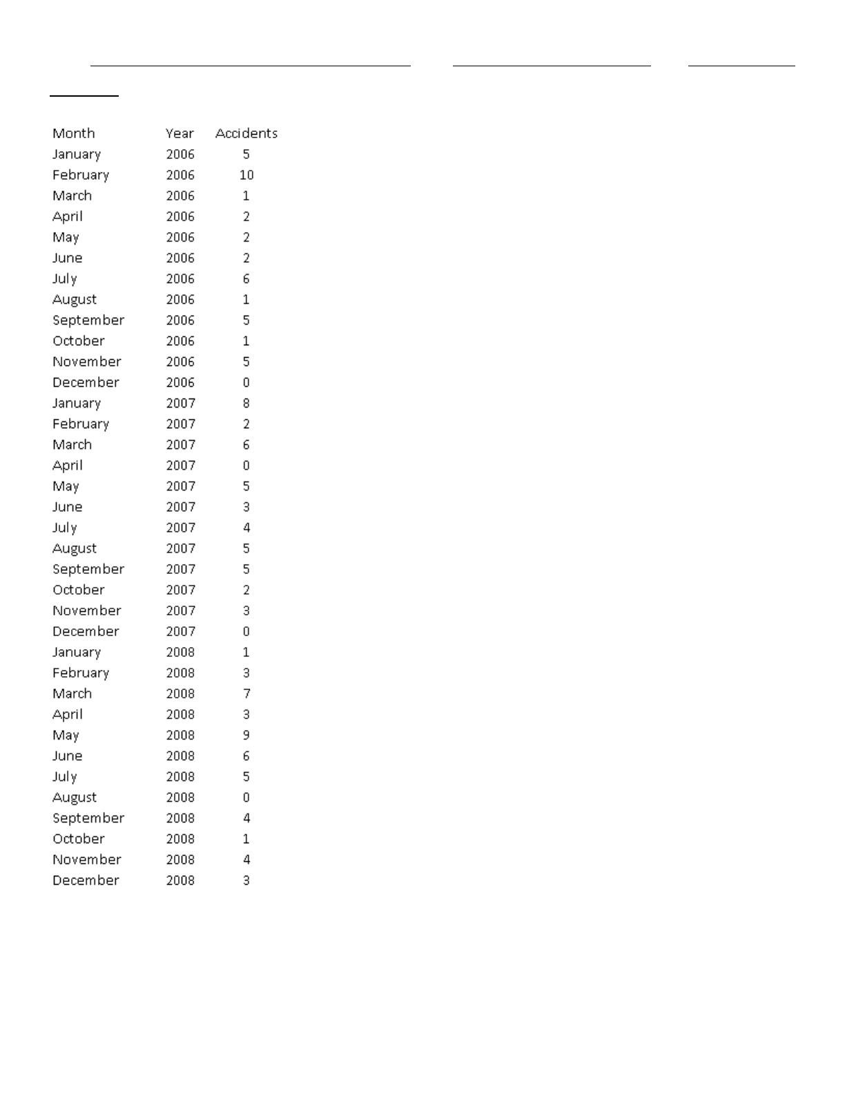
Name:
Class:
Date:
chapter 12
Is this time series random? Perform a runs test and compute a few autocorrelations to support your answer.
The number of employees on the payroll at a computer software company is recorded at the start of each month from
Name:
Class:
Date:
chapter 12
January 2007 to December 2009. These data are shown below.
Year
Jan
Feb
March
April
May
June
July
Aug.
Sept.
Oct.
Nov.
Dec
2007
348
352
330
347
339
370
380
392
400
410
405
367
2008
350
341
345
355
342
350
370
395
410
401
405
365
2009
348
349
350
350
342
377
369
400
410
406
400
370
101. Develop a time series plot of the data. Does the data appear random on the plot?
The table below contains 5 years of monthly data on sales (number of units sold) for a particular company, in
addition to extra columns containing information needed to answer some of the questions. The company
suspects that except for random noise, its sales are growing by a constant percentage each month and that they
will continue to do so for at least the near future.
102. Explain briefly whether the plot of the series visually supports the company’s suspicion.
Suppose that simple exponential smoothing with is used to forecast monthly Pepsi sales at a small grocery store.
After March’s demand is observed, the forecasted demand for April is 5000 cans of Pepsi.
103. At the beginning of April, what is the forecast of June’s Pepsi sales?
104. Rite Aid pharmacy in Big Rapids, Michigan is using simple exponential smoothing to predict monthly birthday card
sales. At the end of October 2004, the pharmacy’s forecast for December 2004 sales was 400. In November, 420 cards
were sold, and during December, 425 cards were sold. At the end of December 2004, what is the pharmacy’s forecast for
the total number of cards that will be sold during March and April of 2005? Use .
The data shown below contains total monthly retail sales (in dollars) a small sporting goods store for the years 2006–
2008.
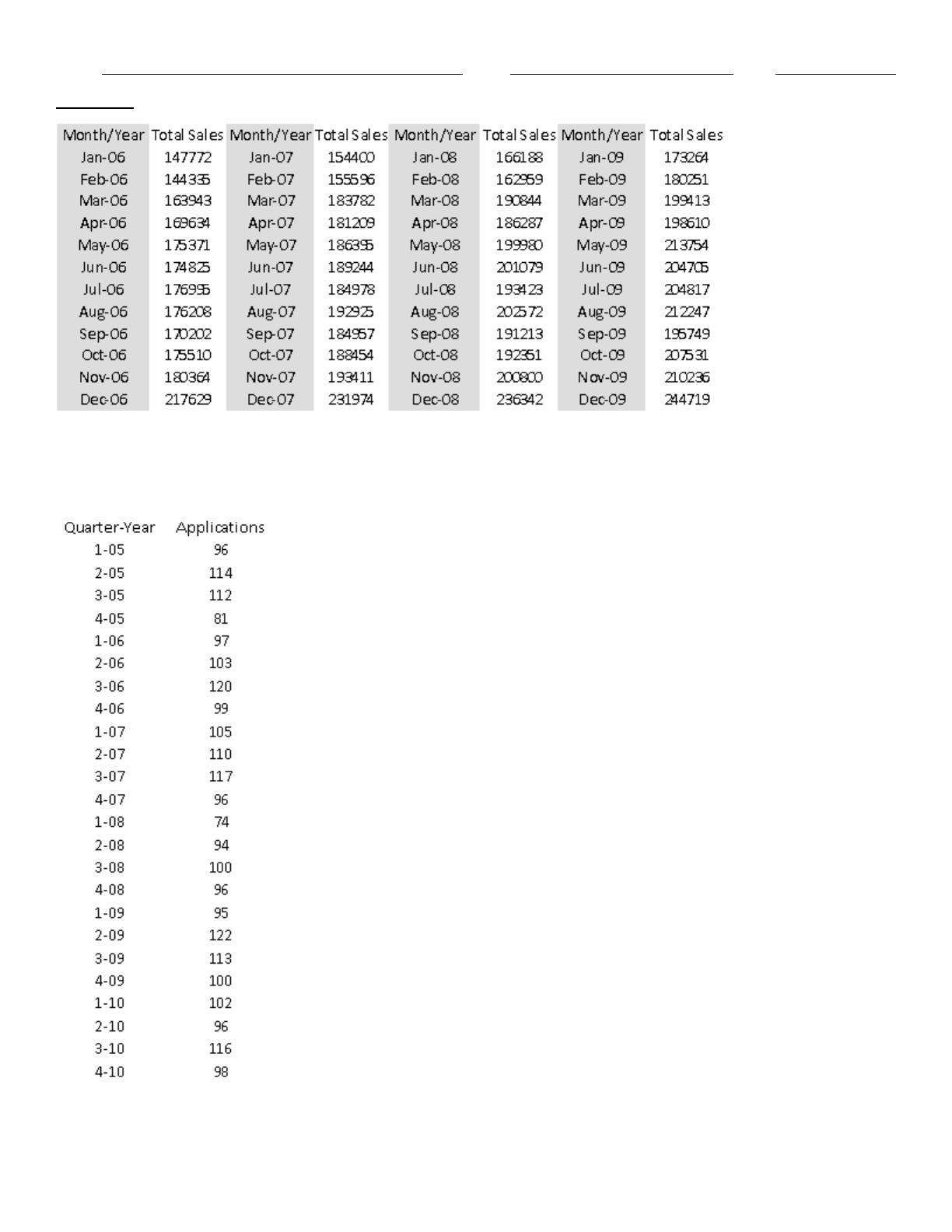
Name:
Class:
Date:
chapter 12
105. What changes, if any, would you suggest to improve the forecast?
The quarterly numbers of applications for home mortgage loans at a branch office of a large bank are recorded in the
table below.
106. (A) Perform a runs test and compute a few autocorrelations to determine whether this time series is random.
(B) Obtain a time series chart. Which of the exponential smoothing models do you think should be used for forecasting

Name:
Class:
Date:
chapter 12
based on this chart? Why?
(C) Use simple exponential smoothing to forecast these data, using no holdout period and requesting 4 quarters of future
forecasts. Use the default smoothing constant of 0.10.
(D) Repeat (C), optimizing the smoothing constant. Does it make much of an improvement?
Name:
Class:
Date:
chapter 12
Answer Key
Name:
Class:
Date:
chapter 12
Name:
Class:
Date:
chapter 12
Name:
Class:
Date:
chapter 12
should give us a high degree of confidence that the forecast is holding up well as we extend past the data.
Name:
Class:
Date:
chapter 12
Name:
Class:
Date:
chapter 12
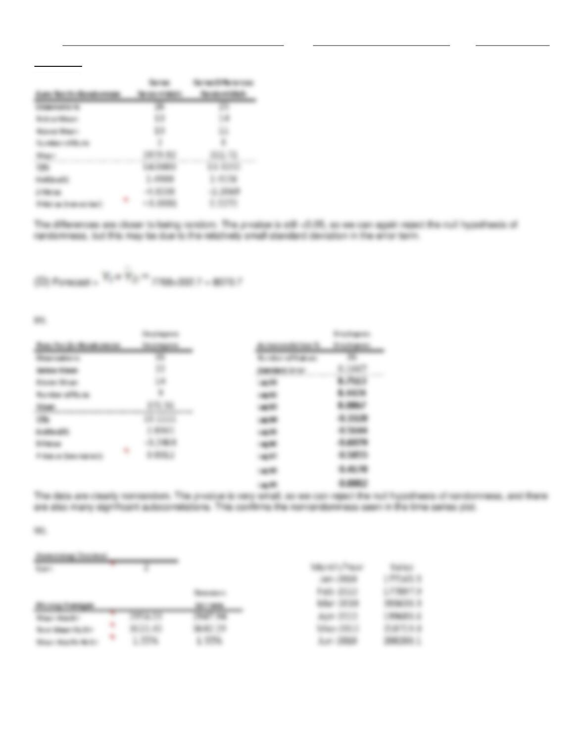
are also many significant autocorrelations. This confirms the nonrandomness seen in the time series plot.
Name:
Class:
Date:
chapter 12
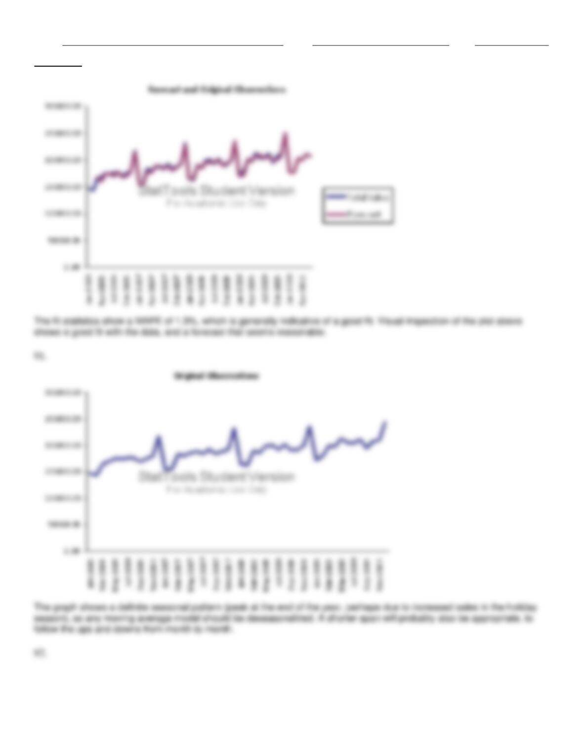
shows a good fit with the data, and a forecast that seems reasonable.
follow the ups and downs from month to month.
Name:
Class:
Date:
chapter 12
Name:
Class:
Date:
chapter 12
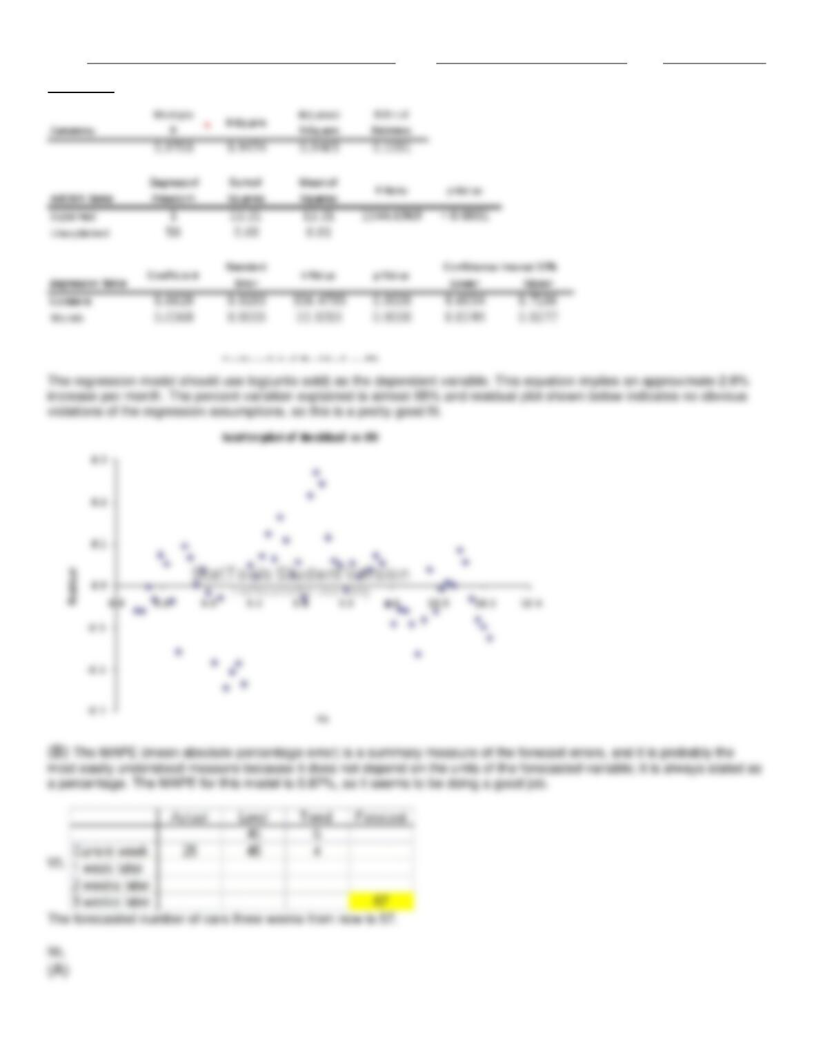
a percentage. The MAPE for this model is 0.87%, so it seems to be doing a good job.
The forecasted number of cars three weeks from now is 57.
Name:
Class:
Date:
chapter 12
Name:
Class:
Date:
chapter 12
previous observation to forecast the next value.
(A) Forecast for July is 4500 bottles.
Name:
Class:
Date:
chapter 12
observation was <4500.
observation was <5000.
randomness), although there is also some mild evidence of negative autocorrelation (more zigzagging than expected).
Name:
Class:
Date:
chapter 12
Name:
Class:
Date:
chapter 12
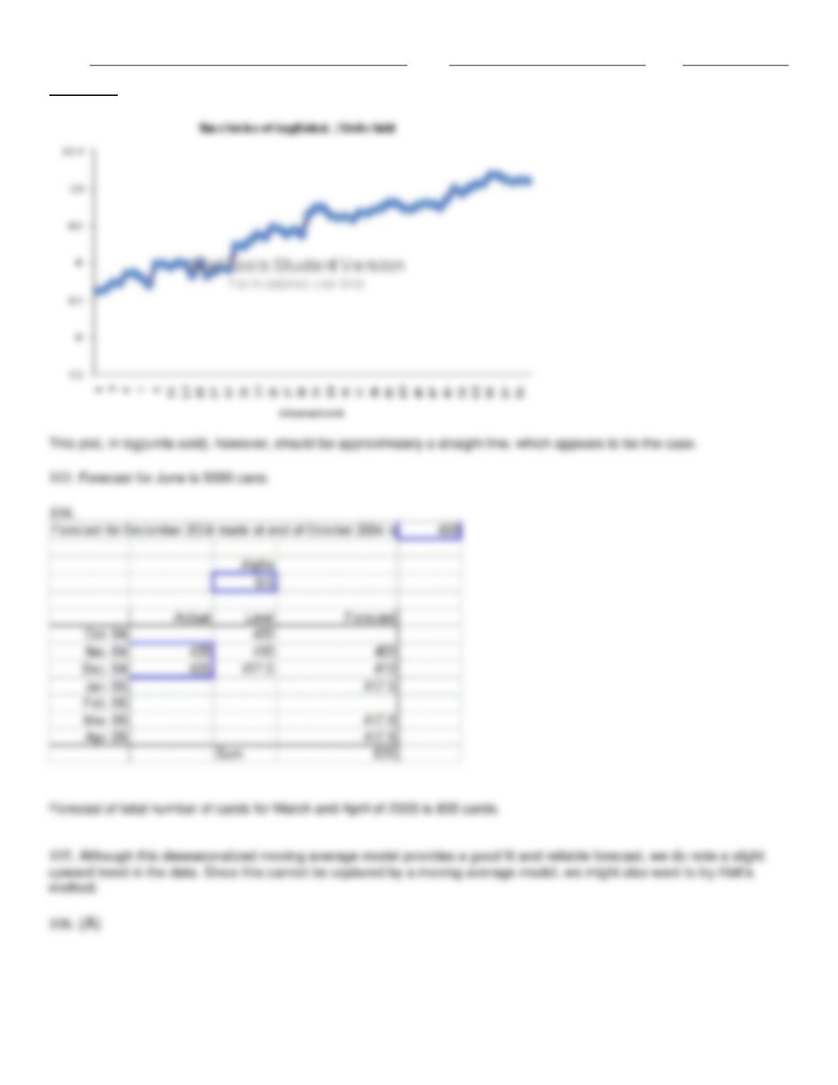
This plot, in log(units sold), however, should be approximately a straight line, which appears to be the case.
method.
Name:
Class:
Date:
chapter 12
(D)
Name:
Class:
Date:
chapter 12