Unlock document.
This document is partially blurred.
Unlock all pages and 1 million more documents.
Get Access
c. Perform an F test and determine whether or not there is a significant relationship
between demand and unit price. Let = 0.05.
d. Perform a t test to determine whether the slope is significantly different from zero.
Let = 0.05.
e. Would the demand ever reach zero? If yes, at what price would the demand be zero.
Show your complete work.
4. A company has recorded data on the daily demand for its product (y in thousands of
units) and the unit price (x in hundreds of dollars). A sample of 15 days demand and
associated prices resulted in the following data.
x = 75
x 2 = 469
y = 135
y 2 = 1315
x y = 616
a. Using the above information, develop the least-squares estimated regression line and
write the equation.
b. Compute the coefficient of determination.
c. Perform an F test and determine whether or not there is a significant relationship
between demand and unit price. Let = 0.05.
d. Would the demand ever reach zero? If yes, at what price would the demand be zero?
5. A company has recorded data on the daily demand for its product (y in thousands of
units) and the unit price (x in hundreds of dollars). A sample of 15 days demand and
associated prices resulted in the following data.
x = 75
x 2 = 437
y = 180
y 2 = 2266
x y = 844
a. Using the above information, develop the least-squares estimated regression line and
write the equation.
b. Compute the coefficient of determination.
c. Perform an F test and determine whether or not there is a significant relationship
between demand and unit price. Let = 0.05.
d. Would the demand ever reach zero? If yes, at what price would the demand be zero?
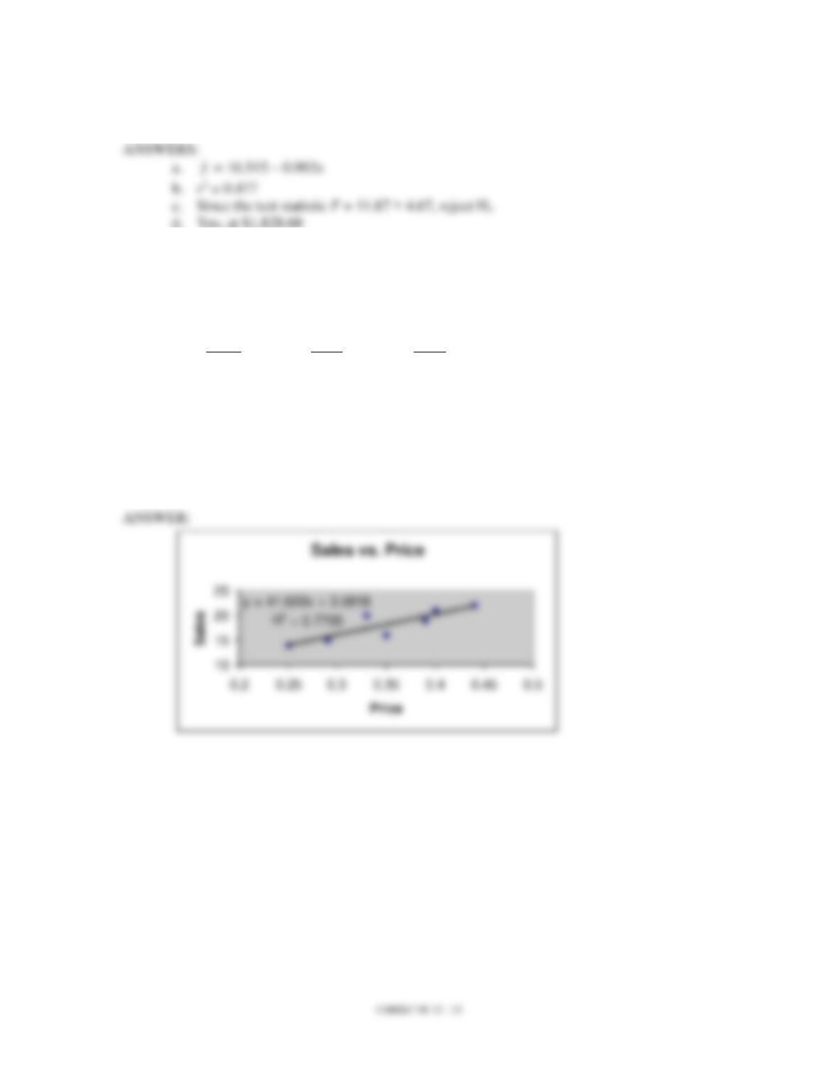
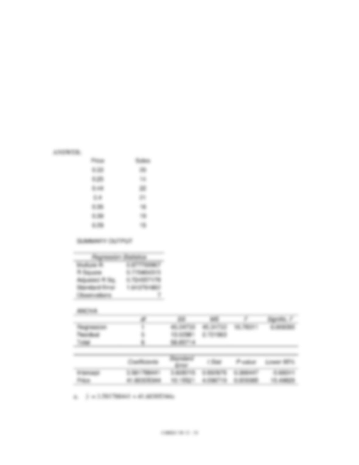
6. A company has recorded data on the weekly sales for its product (y) and the unit price of
the competitor’s product (x). The data resulting from a random sample of 7 weeks
follows. Use Excel to develop a scatter diagram and to compute the least squares
estimated regression equation and the coefficient of determination.
Week
Price
Sales
1
.33
20
2
.25
14
3
.44
22
4
.40
21
5
.35
16
6
.39
19
7
.29
15
7. We are interested in determining the relationship between daily supply (y) and the unit
price (x) for a particular item. A sample of ten days supply and associated price resulted
in the following data.
x = 66
x2= 526
y = 71
y2= 605
xy = 557
a. Develop the least square estimated regression equation.
b. Compute the coefficient of determination and fully explain its meaning.
c. At = 0.05, perform a t-test and determine if the slope is significantly different from
zero.
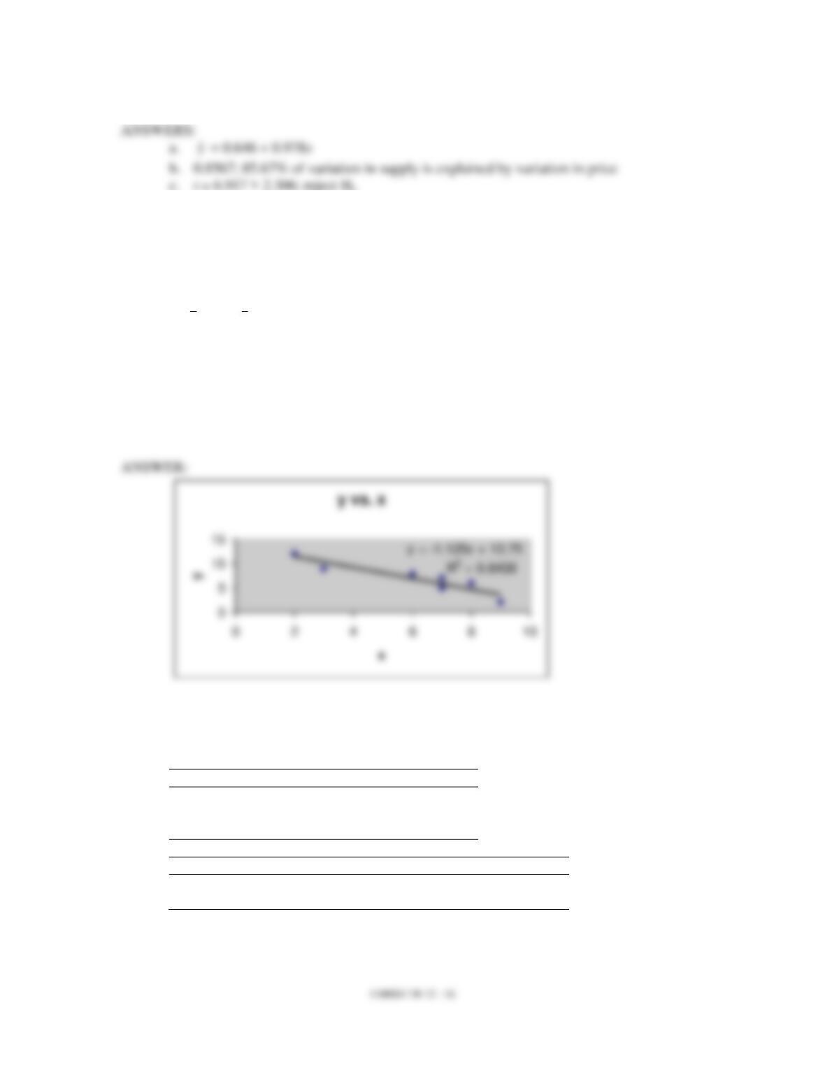
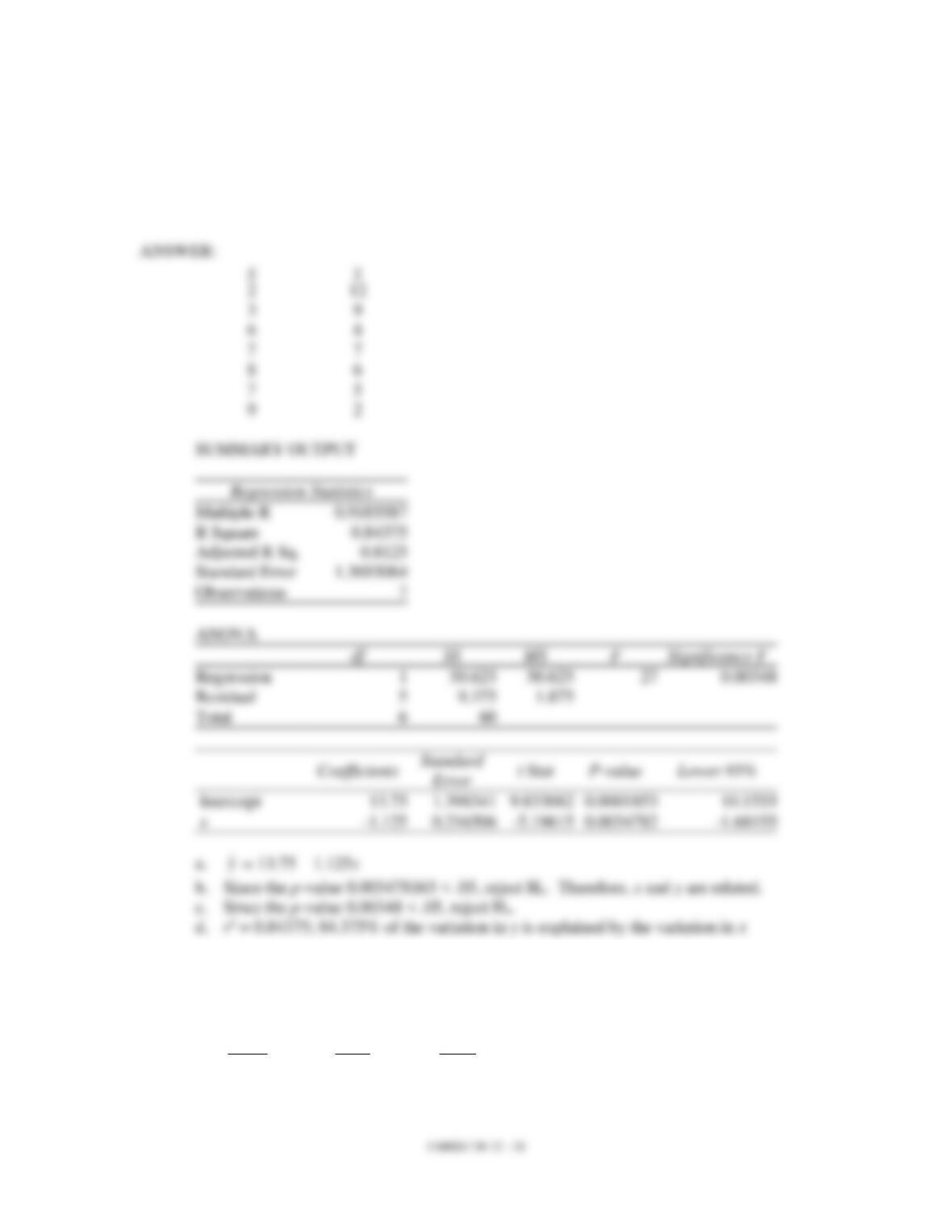
8. Given below are seven observations collected in a regression study on two variables, x
(independent variable) and y (dependent variable). Use Excel to develop a scatter
diagram and to compute the least squares estimated regression equation and the
coefficient of determination.
x
y
2
12
3
9
6
8
7
7
8
6
7
5
9
2
9. Shown below is a portion of a computer output for a regression analysis relating y
(dependent variable) and x (independent variable).
ANOVA
df
SS
Regression
1
50.58
Residual
13
55.42
Total
14
106.00
Coefficients
Standard Error
t Stat
Intercept
16.156
1.42
Variable x
-0.903
0.26
a. Perform a t test and determine whether or not y and x are related. Use = 0.05.
b. Compute the coefficient of determination and fully interpret the meaning. Be very
specific.
10. Shown below is a portion of a computer output for regression analysis relating y
(dependent variable) and x (independent variable).
ANOVA
df
SS
Regression
1
882
Residual
20
4000
Total
21
4882
Coefficients
Standard Error
t Stat
Intercept
5.00
3.56
Variable x
6.30
3.00
a. What has been the sample size for the above?
b. Perform a t-test and determine whether or not x and y are related. Use = 0.05.
c. Perform an F-test and determine whether or not x and y are related. Use = 0.05.
d. Compute the coefficient of determination.
e. Interpret the meaning of the value of the coefficient of determination that you found
in d. Be very specific.
11. Given below are seven observations collected in a regression study on two variables, x
(independent variable) and y (dependent variable). Use Excel’s Regression Tool to
answer the following questions.
x
y
2
12
3
9
6
8
7
7
8
6
7
5
9
2
a. What is the estimated regression equation?
b. Perform a t test and determine whether or not x and y are related. Use = 0.05.
c. Perform an F test and determine whether or not x and y are related. Use = 0.05.
d. Find and interpret the coefficient of determination.
12. A company has recorded data on the weekly sales for its product (y) and the unit price of
the competitor’s product (x). The data resulting from a random sample of 7 weeks
follows. Use Excel’s Regression Tool to answer the following questions.
Week
Price
Sales
1
.33
20
2
.25
14
3
.44
22
4
.40
21
5
.35
16
6
.39
19
7
.29
15
a. What is the estimated regression equation?
b. Perform a t test and determine whether or not x and y are related. Use = 0.05.
c. Perform an F test and determine whether or not x and y are related. Use = 0.05.
d. Find and interpret the coefficient of determination.
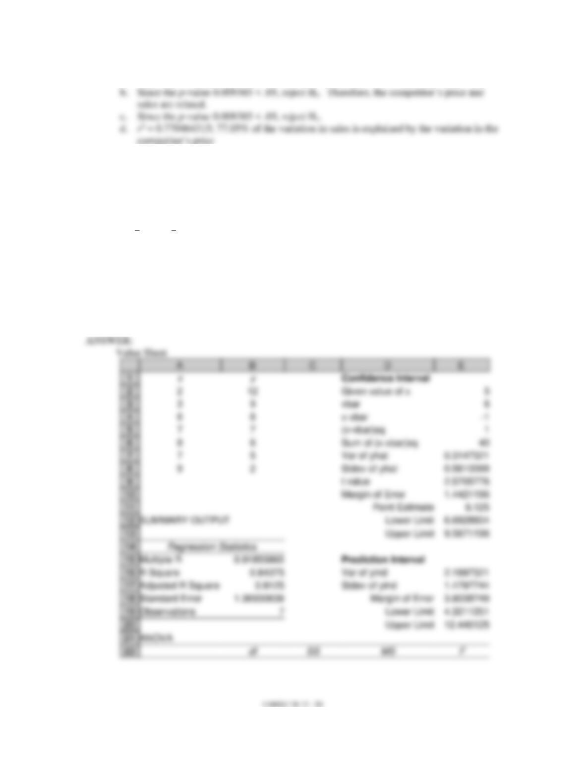
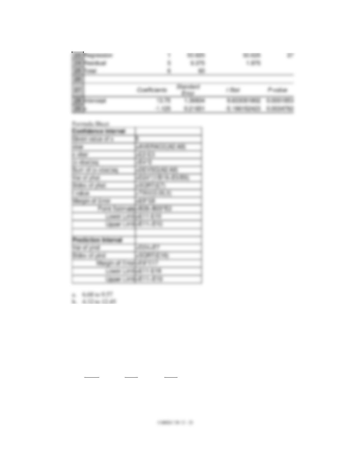
12. Given below are seven observations collected in a regression study on two variables, x
(independent variable) and y (dependent variable). Use Excel to
a. compute a 95% confidence interval for E(y) when x = 5
b. compute a 95% prediction interval for y when x = 5.
x
y
2
12
3
9
6
8
7
7
8
6
7
5
9
2
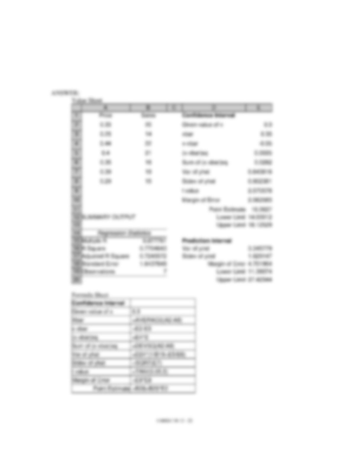
12. A company has recorded data on the weekly sales for its product (y) and the unit price of
the competitor’s product (x). The data resulting from a random sample of 7 weeks
follows. Use Excel to:
a. compute a 95% confidence interval for expected sales for all weeks when the
competitor’s price is .30.
b. compute a 95% prediction interval for sales for a week when the competitor’s price is
.30.
Week
Price
Sales
1
.33
20
2
.25
14
3
.44
22
4
.40
21
5
.35
16
6
.39
19
7
.29
15
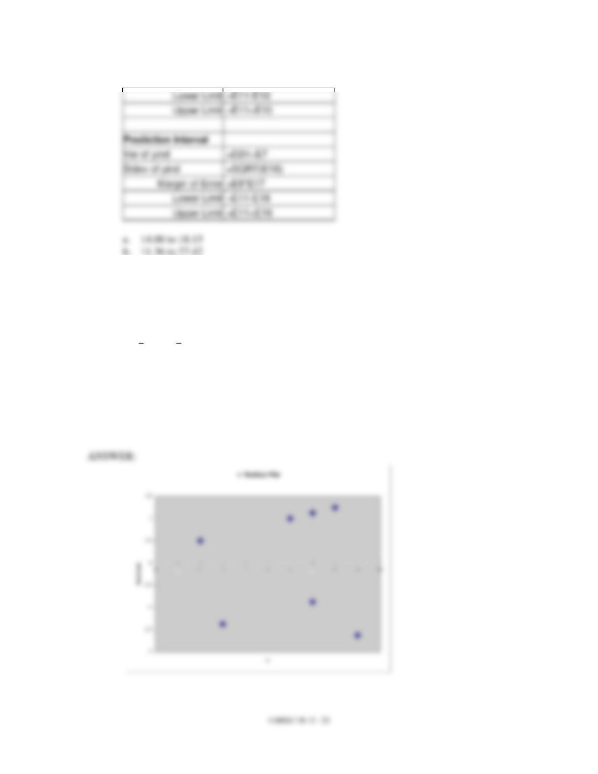
15. Given below are seven observations collected in a regression study on two variables, x
(independent variable) and y (dependent variable). Use Excel’s Regression Tool to
construct a residual plot and use it to determine if any model assumption have been
violated.
x
y
2
12
3
9
6
8
7
7
8
6
7
5
9
2
EMBS4 TB 12 - 24
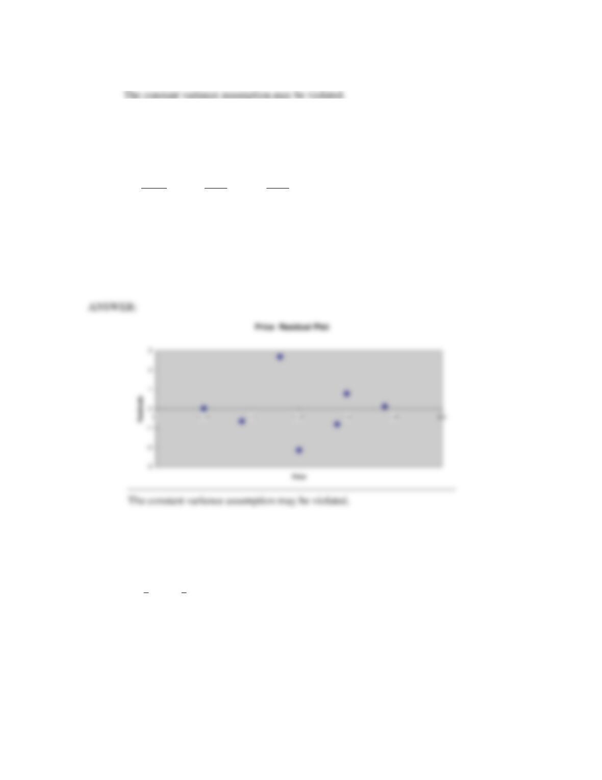
16. A company has recorded data on the weekly sales for its product (y) and the unit price of
the competitor’s product (x). The data resulting from a random sample of 7 weeks
follows. Use Excel’s Regression Tool to construct a residual plot and use it to determine
if any model assumption have been violated.
Week
Price
Sales
1
.33
20
2
.25
14
3
.44
22
4
.40
21
5
.35
16
6
.39
19
7
.29
15
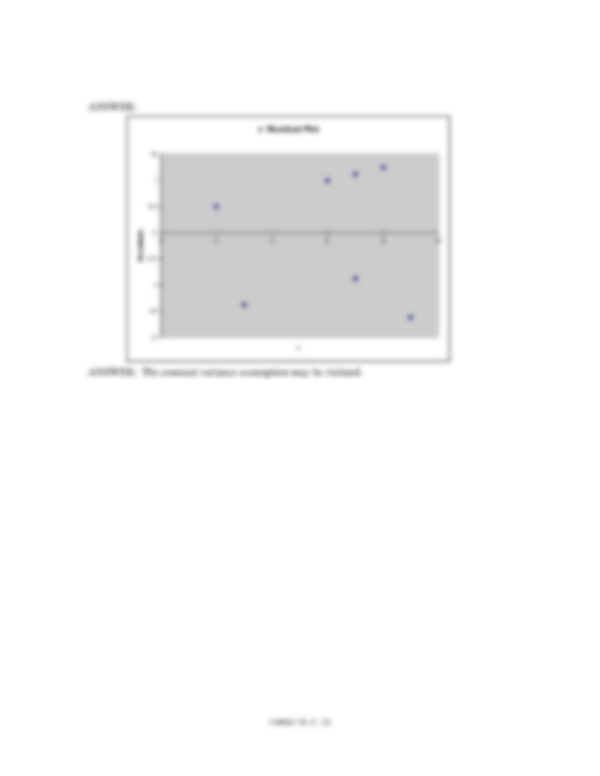
17. Given below are seven observations collected in a regression study on two variables, x
(independent variable) and y (dependent variable). Use Excel’s Regression Tool to
construct a residual plot and use it to determine if any model assumption have been
violated.
x
y
2
12
3
9
6
8
7
7
8
6
7
5
9
2
18. Connie Harris, in charge of office supplies at First Capital Mortgage Corp., would like to
predict the quantity of paper used in the office photocopying machines per month. She
believes that the number of loans originated in a month influence the volume of
photocopying performed. She has compiled the following recent monthly data:
Number of Loans
Originated in Month
Sheets of Photocopy
Paper Used (000's)
45
22
25
13
50
24
60
25
40
21
25
16
35
18
40
25
a. Develop the least-squares estimated regression equation that relates sheets of
photocopy paper used to loans originated.
b. Use the regression equation developed in part (a) to forecast the amount of paper
used in a month when 42 loan originations are expected.
c. Compute SSE, SST, and SSR.
d. Compute the coefficient of determination r2. Comment on the goodness of fit.
e. Compute the correlation coefficient.
f. Compute the mean square error MSE.
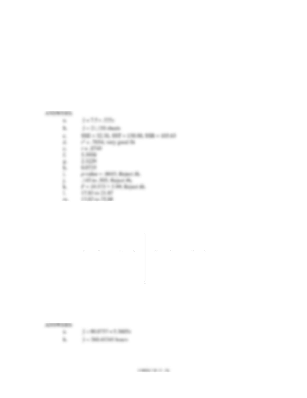
g. Compute the standard error of the estimate.
h. Compute the estimated standard deviation of b1.
i. Use the t test to test the following hypothesis
1 = 0 at
= .05.
j. Develop a 95% confidence interval estimate for
1 to test the hypothesis
1 = 0.
k. Use the F test to test the hypothesis
1 = 0 at a .05 level of significance.
l. Develop a 95% confidence interval estimate of the mean number of sheets of
paper used when 38 mortgages are originated.
m. Develop a 95% prediction interval estimate for the number of sheets of paper
used when 38 mortgages are originated.
19. Scott Bell Builders would like to predict the total number of labor hours spent framing a
house based on the square footage of the house. The following data has been compiled
on ten houses recently built.
Square
Footage
(100s)
Framing
Labor
Hours
Square
Footage
(100s)
Framing
Labor
Hours
20
195
27
225
21
170
29
240
23
220
31
225
23
200
32
275
26
230
35
260
a. Develop the least-squares estimated regression equation that relates framing
labor hours to house square footage.
b. Use the regression equation developed in part (a) to predict framing labor hours
when the house size is 3350 square feet.


