192
Chapter 12 Descriptive statistics
Activities and Resources
To gain competency in the content presented in Chapters 12 and 13, students need to have practice
analyzing data. One way to accomplish this is to use existing datasets available online as referenced in the
Chapter 12 and Chapter 13 activities.
Before turning the class loose on any data analysis practice opportunities on the activity below or
elsewhere, it is a good idea to describe how to open SPSS, and how to enter data. Alternatively, you could
assign reading some introductory information. Many will not know how to use a database or how to ‘get
around’ in SPSS or an alternative statistics package. Pairing less experienced with more experienced
peers works but be careful. It is easy for an able student to move through these exercises quickly and
leave the less able peer in the dust, knowing less than when he started. I have often had my most able
students skip the assignments and instead work with me as a consultant for the other students who get
stuck. If your class is very able you could have them complete the assignment out of class. For those
students who might have their own research data, I have allowed them to use their own data and work
though parallel questions.
Suggested Activity
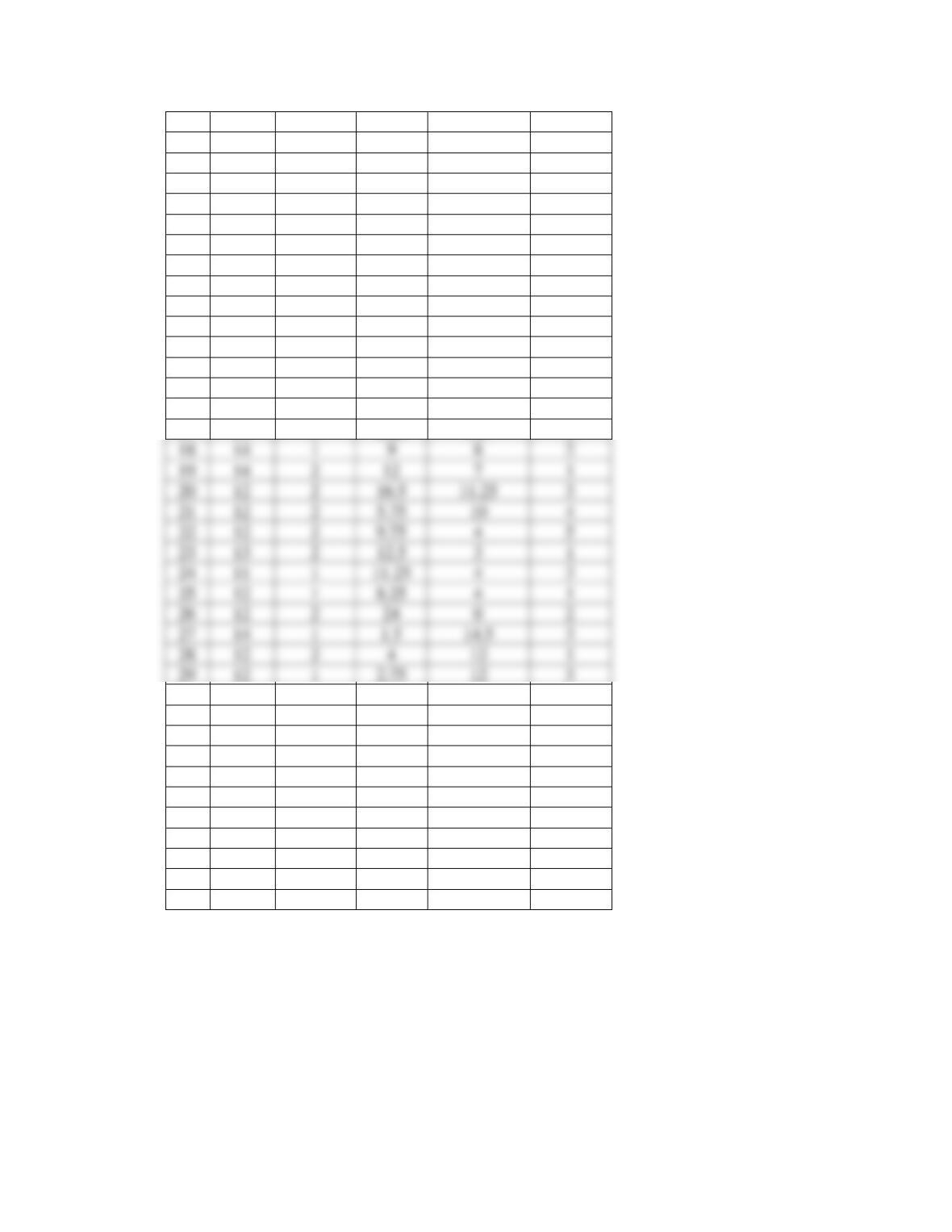
1. To get initial practice entering and analyzing data I have generated a dummy dataset that includes
the following variables for 40 participants: ID number, age, gender, hours spent playing video games in a
given week (Hours), hours spent on exercise in a given week (Exercise), and the number of nights in a
given week that the participants’ families ate dinner together. As a review, ask students to generate two
research questions and corresponding hypotheses for these variables and then share the following activity.
12.1 Doug and David are researchers who examine youth health. Numerous recent studies have
suggested that youth in the 10-15 year old range are increasingly engaged in many hours of video
game playing, they are not active enough (as defined by at least one hour of exercise per day),
ID
AGE
Gender
Hours
Exercise
Dinner
1
12
1
3
14
5
193
2
13
1
14
10
3
3
12
2
12
2
2
4
11
1
6
7
3
5
11
1
2.5
8.5
3
6
12
2
15
6
2
7
13
1
14
5
1
8
12
2
16
6
4
9
12
1
6
8
3
10
12
2
8
9
3
11
12
1
8
12
3
12
14
1
5
14
3
13
13
2
13
12
3
14
13
1
12
3
2
15
12
2
8.5
7
2
16
12
1
7.75
6
4
17
11
1
8.25
5.5
6
30
13
2
14
2.5
4
31
13
1
2.5
13
7
32
14
2
9.25
10
2
33
11
1
8.75
8
3
34
12
1
11.5
7.75
3
35
12
1
12.5
6.5
3
36
13
1
8.25
7
2
37
12
2
7.5
12.25
2
38
12
1
5.75
14
4
39
13
2
6.25
11.5
1
40
11
2
6.5
10.5
2
1. Generate one descriptive research question that can be addressed by Doug and David’s data.
2. Generate one relationship research question that can be addressed by these data.
3. State one null hypothesis that can be tested with these data.
18
14
1
9
8
2
19
14
2
12
7
1
20
12
2
16.5
11.25
3
21
12
2
5.75
10
4
22
12
2
9.75
4
5
23
13
2
12.5
3
1
24
11
1
4
3
25
12
1
8.25
4
1
26
12
2
24
0
2
27
14
1
1.5
14.5
3
28
12
2
4
12
1
29
12
1
2.75
12
3
194
4. Identify the level of measurement for each of the following variables: Age (reported in
years), Gender (reported as Female=1; Male=2), Hours of video game playing in the week
(reported to the quarter hour), Exercise (reported to the quarter hour), Dinners taken together
as a family (0-7 dinners in the week).
5. Please enter the data into a file after double-checking for accuracy.
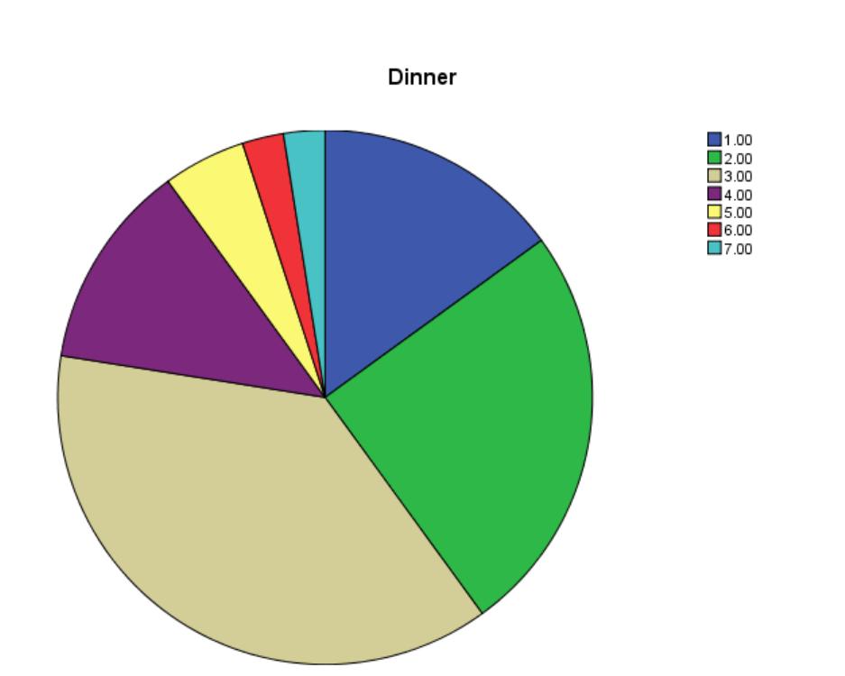
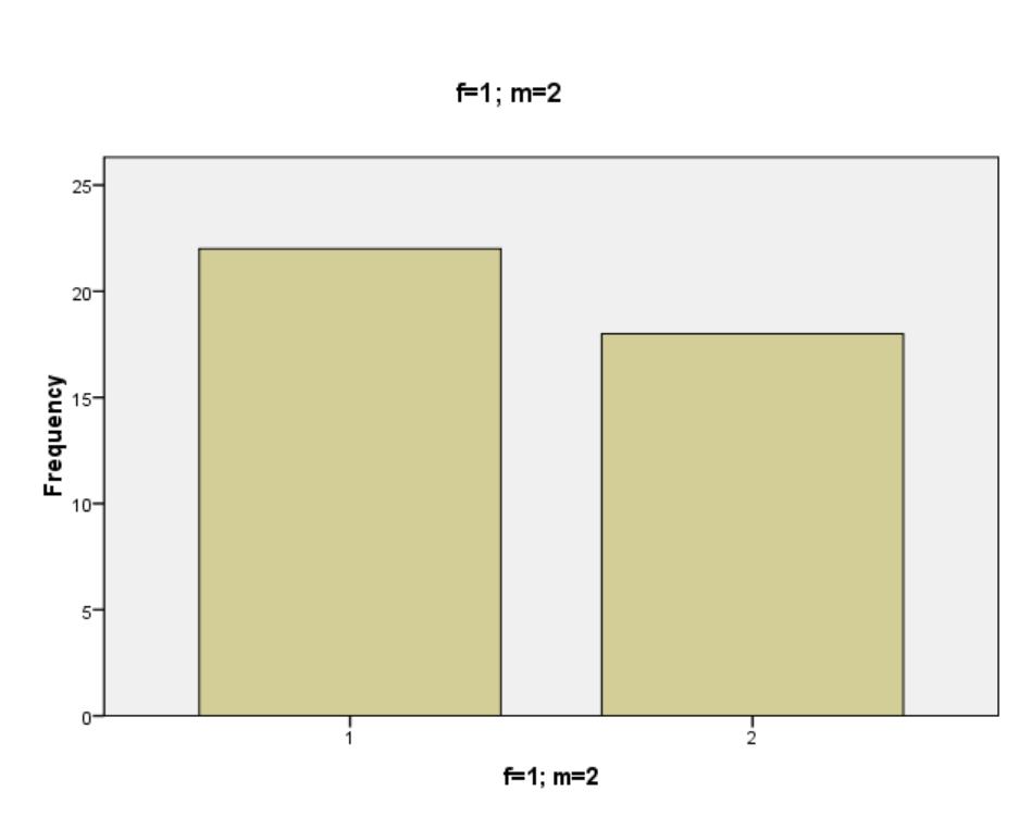
8. Graph the dinner (pie chart) and gender (histogram) data. Graph age, hours of game playing,
and hours of exercise data with frequency distributions.
Handout 12.1 (answers)
1. Generate one descriptive research question that can be addressed by Doug and David’s data.
2. Generate one relationship research question that can be addressed by these data.
3. State one null hypothesis that can be tested with these data.
4. Identify the level of measurement for each of the following variables: Age (reported in years),
Gender (reported as Female=1; Male=2), Hours of video game playing in the week (reported to
5. Please enter the data into a file after double-checking for accuracy.
6. Please provide descriptive information for all of the variables. Which is the best measure of
central tendency for each variable? Why? As categorical data, Gender should be reported by
195
196
Exercise
Frequency
Percent
Valid Percent
Cumulative
Percent
Valid
0
1
2.5
2.5
2.5
2
1
2.5
2.5
5.0
2.5
1
2.5
2.5
7.5
3
2
5.0
5.0
12.5
4
3
7.5
7.5
20.0
5
1
2.5
2.5
22.5
5.5
1
2.5
2.5
25.0
6
3
7.5
7.5
32.5
6.5
1
2.5
2.5
35.0
7
4
10.0
10.0
45.0
7.75
1
2.5
2.5
47.5
8
3
7.5
7.5
55.0
8.5
1
2.5
2.5
57.5
9
1
2.5
2.5
60.0
10
Statistics
7.5
7.5
67.5
10.5
Hours
Exercise
11.25
N
Valid
40
40
11.5
Missing
0
0
12
Mean
9.2250
8.1938
12.25
Median
8.3750
8.0000
13
Mode
8.25a
7.00a
14
Std.
Deviation
4.63051
3.78911
14.5
Range
22.50
14.50
Total
a. Multiple
modes exist.
The smallest
value is
shown
100.0
100.0
197
Group Statistics
f=1;
m=2
N
Mean
Std. Deviation
Std. Error Mean
Exercise
1
22
8.7159
3.65661
.77959
2
18
7.5556
3.95429
.93204
Hours
1
22
7.6591
3.82780
.81609
2
18
11.1389
4.90290
1.15562
Dinner
Frequency
Percent
Valid Percent
Cumulative
Percent
Valid
1
6
15.0
15.0
15.0
2
10
25.0
25.0
40.0
3
15
37.5
37.5
77.5
4
5
12.5
12.5
90.0
5
2
5.0
5.0
95.0
6
1
2.5
2.5
97.5
7
1
2.5
2.5
100.0
Total
40
100.0
100.0
7. Are there more girls or boys in the sample? On average, do youth in the sample play more time
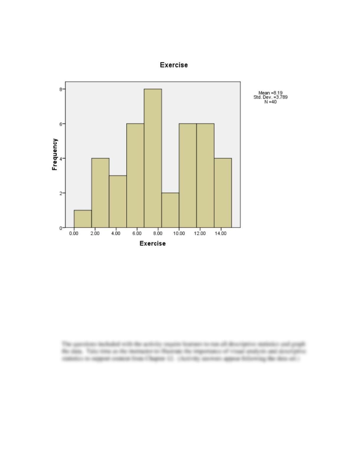
8. Graph the dinner (pie chart) and gender (histogram) data. Graph age, hours of game playing, and
hours of exercise data with frequency distributions. (Examples of some follow)
198
199
200
2. I usually have them work in pairs and this activity takes a long time. Schedule a computer lab if
you do not have access to computers in the classroom setting. A dataset (complete with problems
and questions) for the students to enter is presented below. Students will make mistakes. They
will, for example, enter height as 64 for 6 foot 4 inches. They will enter nominal data as ratio and
will elect to or not elect to throw ‘errors’ in the data out. These choices are important for them to
make and provide the instructor opportunities to illustrate data management and data cleaning
strategies.
The questions included with the activity require learners to run all descriptive statistics and graph
Have the students complete the following tasks:
1. Please enter your data into a data file and turn in a data description and code sheet.
201
2. Please graph the descriptive information for each of the variables. You must use at least 2
different types of graphs or visual displays.
3. Turn in a copy of the graphs and the data file.
4. What is the average age of the class?
5. What is the average number of hours of exercise per week?
6. Was HS GPA or College GPA higher?
7. How many children do the class members have total?
8. How many members of our class are single children?
9. Provide printouts of graphed data for gender and martial status.
Tool to collect data. Have each student collect three cases.
Gender________________ College GPA______________
Age___________________ Number of siblings____________
Height_________________ Marital status_______________
Weight________________ Number of children __________
High school GPA ________________ Exercise per week(hr)____________
Example dataset
Gen age ht wt HSgpa Cgpa siblings marital children exercise
male 21 6’1’’ 190 2.4 2.0 4 single none 10 hour
female 21 5’5” 135 3.2 3.0 3 single none 3
female 18 5.51/2 135 3.5 2.5 2 single none 5
f 24 5’4’ 210 3.96 2.73/3.11 5 s 0 0
F 48 5’7’ 117 2.9 3 M 2 3
m 52 5’8’ 145 2.9 3.3/4.0 1 W 2 15
m 48 6FT 190 3.6 3.8 2 D 2 6
F 48 5’2’ 200 3.7 3.7 4 D 1 0
M 40 6’4’ 185 3.2 3.5 0 M 3 2
202
female 38 5’3’ 127 3.5 3.65 1 divorced 3 0 hours
male 23 5’11 180 3.75 3.78 6 single 0 0
female 39 5’6 145 3.554 n/a 1 married 1 3 hours
female 29 5’6 145 3.0 3.0 2 married 5 hours
female 32 5’9 160 3.0 3.0 3 married 1 0
male 25 5’9 210 2.8 2.3 0 single 0 10hrs
female 48 5’6 142 3.5 4.0 8 married 2 3 hrs
female 31 5’6 135# 3.95 3.82 2 married 1 5
female 25 5’3 140 3.76 3.82 4 married 1 3
female 56 5’2 136 ?/3.7 3.5 4 M 2 3
f 26 5’3 133 3.5 3.2 2 M 1 3
M 25 5’11 190 3.8 3.6 3 S 0 7
F 24 5’2 140 3.7 3.45 2 S 0 10.5
M 29 5ft11in 225lbs 3.46 3.80 4 single 0 2
Male 48 5ft10in 215lbs 2.13 2.25 1 divorced 0 1
Female 30 5ft9in 250lbs 3.25 3.46 2 divorced 0 3
male 23 6’ 200lbs 3.94 4.0 1 S 0 3
F 22 5’3 140 3.35 3.25 1 S 0 1
F 2.5 5’2 160 3.2 2.9 1 S 0 2
male 34 6’2 150 3.2 2.97 2 S 1 1
male 37 5’11 175 3.4 3.0 2 M 2 1/2hr
female 36 5’8 165 2.6 3.9 2 M 3 1/2hr
female 23 5’5 126 2.3 3.1 0 single 1 0
female 31 5’3 134 2.7 3.4 1 single 0 3
female 38 5’1 202 5.2 3.89 8 single 1 0
F 37 5’4 135 3.76 4.0 1 S 0 4
F 21 5’5 125 3.4 3.3 1 S 0 6
M 20 5’11 160 2.9 3.1 2 S 0 5
F 30 5’3 115 3.85 3.875 0 single 0 0
M 49 6’0’ 250 2.5 3.0 1 married 2 6
F 44 5’8 150 3.5 3.65 3 married 2 0
Female 36 5’5 120lbs 3.6 3.6 1 M 1 1
Female 30 5’4.5” 185lbs 3.2 3.0 1 M 1 3
female 31 5’7” 145lbs 4.0 3.75 1 M 0 3
male 22 f’11 170 3.3 2.8 3 single none 10hrs
male 26 5’10 150 3.8 3.2 4 single 0 10 hrs
female 32 5’5 100 2.8 3.8 0 single 0 0
F 36 5’6 265 2.2 NA 3 married 4 2
203
Chapter 12 Activity 2 Answers
The included dataset allows for opportunities to discuss aspects of instrument design, data entry, and
analysis concerns. The instructor can either discuss up front things to think about as a class or one can let
them figure it out and discuss it along the way.
Please note that the answers found for the Chapter 12 questions will differ depending upon data entry
decisions made by the student. If you are having students enter the data have them follow the following
steps:
• First, give each case a sequential number and write it on the hardcopy. This will allow you to
discuss them by case number if needed.
• Six, double check and then examine through descriptives
Decisions and notes about the data from which the answers are provided
Female is 1, Male is 2
Marital status is: single is 1, married is 2, divorced is 3, widowed is 4, N/A is dropped
Cases with more than one GPA—the first was used
f’11 was entered as 5’11
1-2 hours was represented by 1.5
To save ink and given that printer space is usually limited I collect this assignment either
electronically or saved to diskette.
1. Please enter your data into a data file and turn in a data description and code sheet.
204
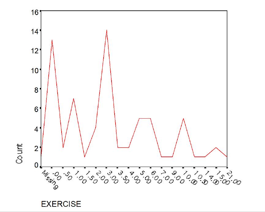
2. Please graph the descriptive information for each of the variables. You must use at least
2 different types of graphs.
3. Turn in a copy of the graphs and the data file.
4. What is the average age of the class?
5. What is the average number of hours of exercise per week?
6. Was HS GPA or College GPA higher?
7. How many children do the class members have total?
8. How many members of our class are single children?
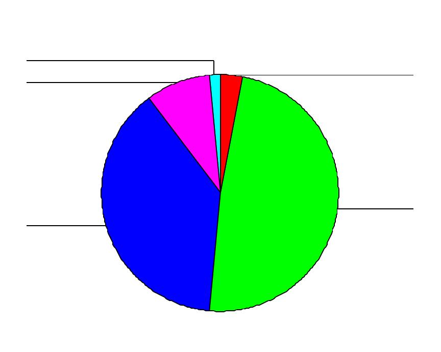
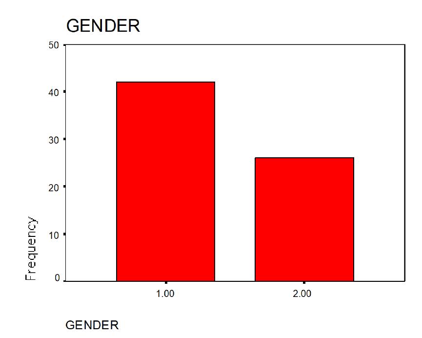
9. Provide printouts of graphed data for gender and martial status.
205
Statistics
GENDER
Frequency
Percent
Valid
Percent
Cumulative Percent
Valid
1.00
42
61.8
61.8
61.8
2.00
26
38.2
38.2
100.0
Total
68
100.0
100.0
MARITAL
Frequency
Percent
Valid
Percent
Cumulative
Percent
Valid
1.00
33
48.5
50.0
50.0
2.00
26
38.2
39.4
89.4
3.00
6
8.8
9.1
98.5
4.00
1
1.5
1.5
100.0
Total
66
97.1
100.0
Missing
System
2
2.9
Total
68
100.0
Descriptive Statistics
N
Minimum
Maximum
Mean
Std.
Deviation
Variance
AGE
67
18.00
65.00
31.7761
10.1680
103.389
HEIGHT
68
60.00
77.00
67.3235
3.9998
15.998
WEIGHT
68
90.00
265.00
162.5000
40.6494
1652.373
HS_GPA
66
2.00
5.20
3.2850
.5549
.308
C_GPA
66
2.00
4.00
3.3053
.5034
.253
SIBLINGS
68
.00
8.00
2.1618
1.7416
3.033
CHILDRE
N
66
.00
6.00
.9848
1.3416
1.800
EXERCISE
67
.00
21.00
4.0448
4.3421
18.854
Valid N
(listwise)
61
GENDER
MARITAL
N
Valid
68
66
Missing
0
2
Mode
1.00
1.00
Range
1.00
3.00
Sum
94.00
107.00
206
Statistics
AGE
HEIGHT
WEIGHT
HS_GPA
C_GPA
SIBLINGS
CHILDRE
N
EXERCIS
E
N
Valid
67
68
68
66
66
68
66
67
Missing
1
0
0
2
2
0
2
1
Mean
31.7761
67.3235
162.5000
3.2850
3.3053
2.1618
.9848
4.0448
Median
30.0000
67.0000
150.0000
3.4000
3.3500
2.0000
.0000
3.0000
Mode
31.00
71.00
135.00
3.50
3.00
1.00
.00
3.00
Std.
Deviation
10.1680
3.9998
40.6494
.5549
.5034
1.7416
1.3416
4.3421
Variance
103.3885
15.9982
1652.3731
.3079
.2534
3.0331
1.7998
18.8540
Range
47.00
17.00
175.00
3.20
2.00
8.00
6.00
21.00
Sum
2129.00
4578.00
11050.00
216.81
218.15
147.00
65.00
271.00
a Multiple modes exist. The smallest value is shown
HEIGHT
Frequency
Percent
Valid
Percent
Cumulative
Percent
Valid
60.00
1
1.5
1.5
1.5
61.00
3
4.4
4.4
5.9
62.00
4
5.9
5.9
11.8
63.00
6
8.8
8.8
20.6
64.00
4
5.9
5.9
26.5
64.50
1
1.5
1.5
27.9
65.00
6
8.8
8.8
36.8
65.50
1
1.5
1.5
38.2
66.00
6
8.8
8.8
47.1
66.50
1
1.5
1.5
48.5
67.00
3
4.4
4.4
52.9
67.50
1
1.5
1.5
54.4
68.00
4
5.9
5.9
60.3
69.00
5
7.4
7.4
67.6
70.00
3
4.4
4.4
72.1
71.00
7
10.3
10.3
82.4
72.00
6
8.8
8.8
91.2
73.00
3
4.4
4.4
95.6
74.00
1
1.5
1.5
97.1
76.00
1
1.5
1.5
98.5
77.00
1
1.5
1.5
100.0
Total
68
100.0
100.0
207
208
4.00
3.00
2.00
1.00
Missing
209
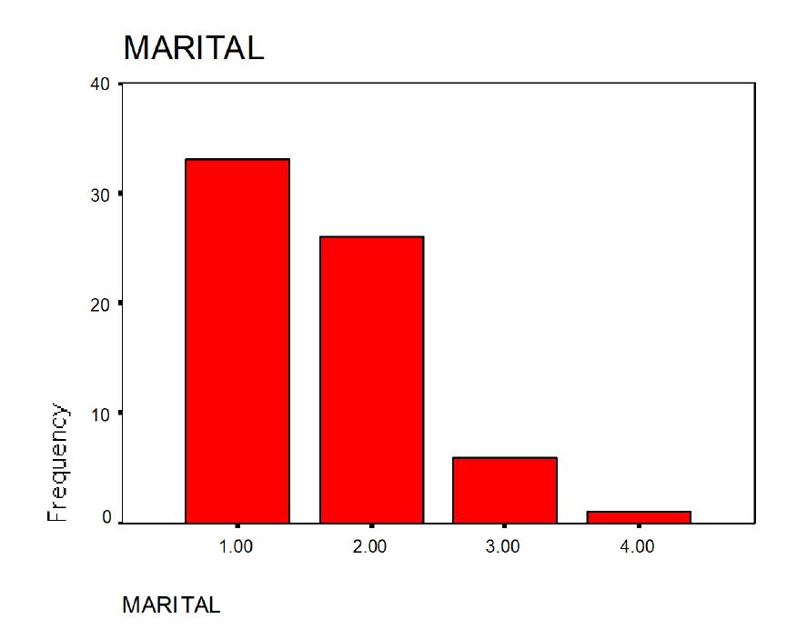
210
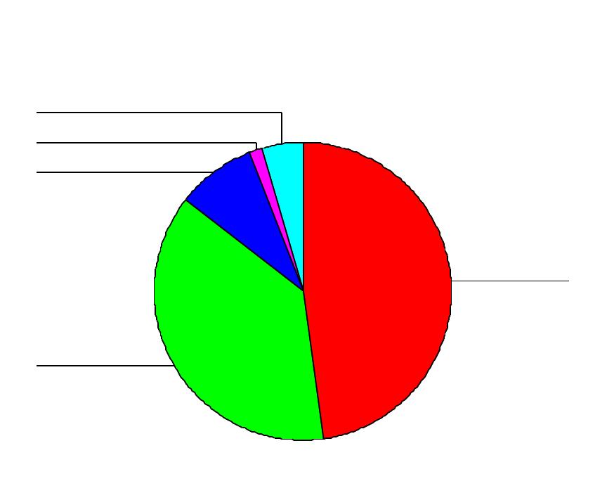
211
MARITAL
Missing
4.00
3.00
2.00
1.00
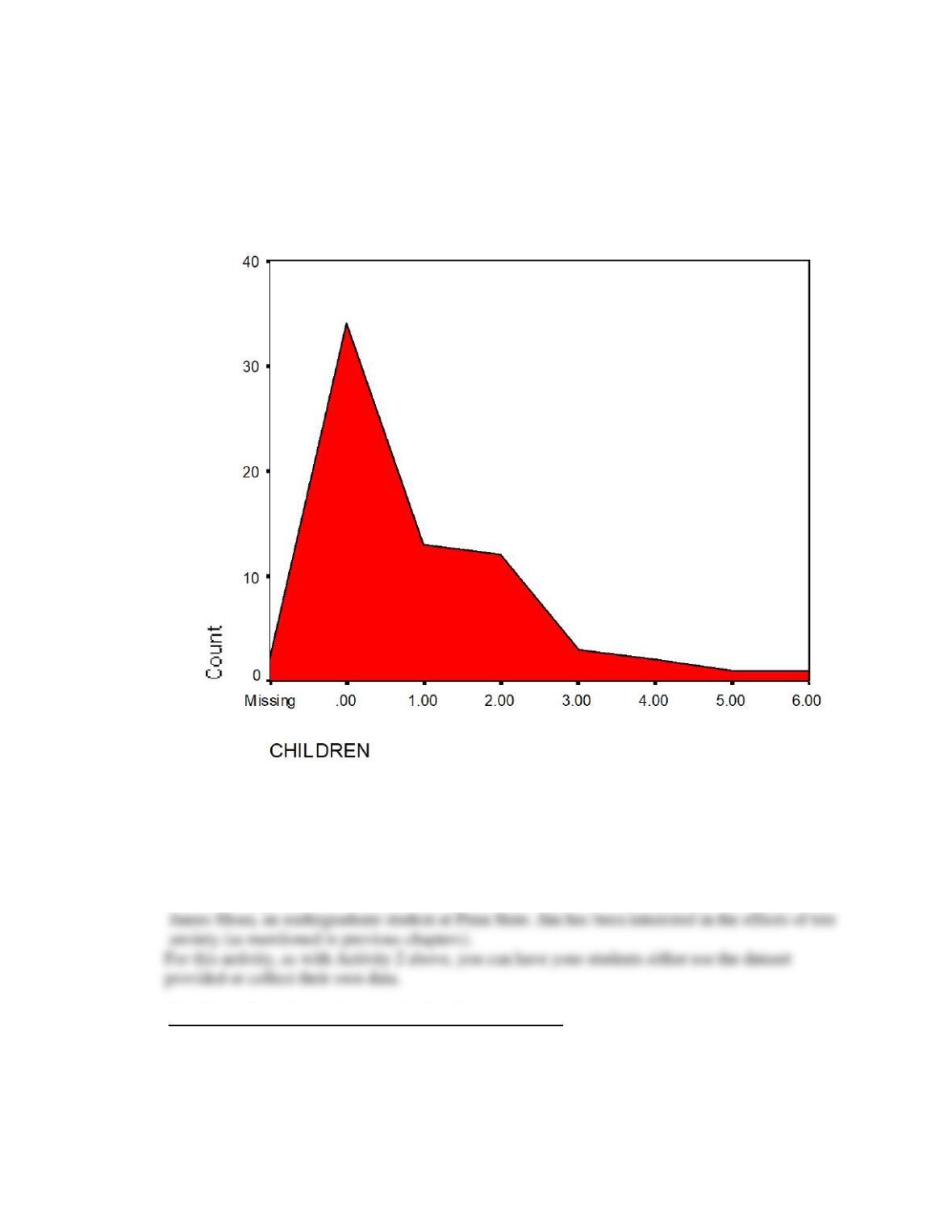
212
3. As a third example, your appendices (Appendix B presents the data in Excel) include a second,
somewhat larger, dataset. I created this dataset based upon a survey (Appendix A) developed by
All missing variables are represented as ‘blank’
No items have been reverse-coded.

213
Id is the participants’ researcher provided id number
GPA is on a four point scale and reported to 2 digits
Class standing is 1=First year; 2= Sophomore, 3=Junior; 4=Senior; 5=Post Graduate
Gender F=1; M=2
SAT is the Math Verbal combined score
Class grade is on a 8=A; 7=A-; 6=B+; 5=B; 4=B-; 3=C+; 2=C; 1=D; 0=F
Test type= 1=MC; 2=Essay; 3=SA; 4=Mix of items
Items are presented by item 3 number. None are reverse-coded.
Anxiety scale represents the sum or the items.
Have the students complete the following tasks:
1. Please run descriptives for each of the variables.
a. For GPA and SAT provide the means, standard deviations, mode, standard error of the
mean, and range
b. For gender, class grade, class standing, and test type provide frequency distributions.
What is the modal value for class grade?
2. Present a graphical display for test type
3. What is the average SAT of the sample?
4. Describe the distribution of the GPA variable.
5. How many sophomores were there in the sample? Seniors?
6. Were there more men or women in the sample?
Activity 12.3 Answers
1. Please run descriptives for each of the variables.
a. For GPA and SAT provide the means, standard deviations, standard error of the
mean, median, and range
Descriptives
b. For Gender, Class grade, class standing, and test type provide frequency
distributions. What is the modal value for Class Standing?
Descriptive Statistics
50 690.00 960.00 1650.00 1200.0000 18.9177 133.76800
50 2.00 2.00 4.00 3.2296 .0665 .47020
50
SAT
GPA
Valid N (listwise)
Statistic Statistic Statistic Statistic Statistic Std. Error Statistic
N Range Minimum Maximum Mean Std.
Deviation
214
Frequencies
Frequency Table
Statistics
50 50 49 50
0 0 1 0
2 8 2 1
Valid
Missing
N
Mode
GENDER Class Grade
Class
Standing Test Type
GENDER
18 36.0 36.0 36.0
32 64.0 64.0 100.0
50 100.0 100.0
1
2
Total
Valid Frequency Percent
Valid
Percent
Cumulative
Percent
Class Grade
1 2.0 2.0 2.0
7 14.0 14.0 16.0
3 6.0 6.0 22.0
2 4.0 4.0 26.0
10 20.0 20.0 46.0
7 14.0 14.0 60.0
6 12.0 12.0 72.0
14 28.0 28.0 100.0
50 100.0 100.0
1
2
3
4
5
6
7
8
Total
Valid Frequency Percent
Valid
Percent
Cumulative
Percent
215
Most students (modal value) are Sophomores
2. Present a graphical display for test type.
Graph
Class Standing
3 6.0 6.1 6.1
33 66.0 67.3 73.5
6 12.0 12.2 85.7
5 10.0 10.2 95.9
1 2.0 2.0 98.0
1 2.0 2.0 100.0
49 98.0 100.0
1 2.0
50 100.0
1
2
3
4
5
8
Total
Valid
SystemMissing
Total
Frequency Percent
Valid
Percent
Cumulative
Percent
Test Type
27 54.0 54.0 54.0
13 26.0 26.0 80.0
10 20.0 20.0 100.0
50 100.0 100.0
1
2
3
Total
Valid Frequency Percent
Valid
Percent
Cumulative
Percent
Test Type
321
Count
30
20
10
0
216
3. What is the average SAT of the sample?
1200
4. Describe the distribution of the GPA variable.
Graph
The distribution is negatively skewed.
5. How many sophomores were there in the sample? Seniors?
This information comes from the Frequency table above for 1b. There were 33
Sophomores and 5 Seniors. The difference is 28 more sophomores.
6. Were there more men or women in the sample?
The student can answer this by the Frequency table above for 1b. A pie graph also
shows this data below. More Men (n=32) Women (n=18)
Graph
GPA
4.003.753.503.253.002.752.502.252.00
12
10
8
6
4
2
0
Std . Dev = . 4 7
Mean = 3.23
N = 50.00
2
1
217
4. Visual analysis is a critical step in descriptive statistics and as a foundation for higher-order
statistics. I often take the time to remind students that different visual representations are
appropriate for different types of data. As a review for creating graphs, you might look through
YouTube videos. There are HUNDREDS of examples of how to do graphing in SPSS. SAS.
EXCEL, and other packages. Many provide great screen shots. I have posted several links to my
class discussion board and students enjoy viewing them at their leisure. The SPSS graphics
tutorial is a great resource since there are now numerous ways to graph the same data.

218
Chapter 12 Test Items
1. Statistical formulas use _____________ letters as shorthand.
a. Greek
b. Latin
c. Capital
d. Ordinal
• 2. Kari’s research study measured the effects of cooperative learning on learners’ ability to
solve complex problems. After scoring the problems and entering the data, her advisor told
her she must have another researcher score the problems. Interestingly, the scores she gave
the participants did not match the scores that the other researcher gave. Kari’s scoring
problem is indicative of a problem with
a. internal consistency reliability.
b. inter-rater reliability.
c. content validity.
d. consequential validity.
3. Machine-scored data can best assist with
a. the validity of the assessment.
b the reliability of the assessment.
c. the reliability of the scoring.
d. the validity of the scoring.
4. Tabulation of data refers to
a. initial organization of quantitative data.
b. final ‘counts’ of qualitative data.
c. initial inferential statistics.
d. creating manuscript tables after analysis.
5. If data are categorical, tabulation includes
a. creating graphs.
b. coding responses.
c. counting responses.
d. statistical analysis.
6. The first step in coding data is
a. determining how categorical data will be coded.
b. determining how many digits are necessary for each variable.
c. giving all participants an ID number.
d. running descriptive statistics for all variables.
7. When calculating a frequency polygon, the first step is to
a. list all scores.
b. calculate means and standard deviations.
c. determine if the distribution is normal.
d. calculate descriptive statistics.
8. Quantitative indices calculated for an entire population are referred to as
a. statistics.
b. inferential.

219
c. parameters.
d. correlations.
9. Quantitative indices calculated for a sample drawn from a population are referred to as
a. statistics.
b. inferential.
c. parameters.
d. statistics.
• 10. Francis wants to present the average mathematics score attained by the participants in her
study. She needs to report a measure of
a. dispersion index.
b. variability.
c. central tendency.
d. relative position.
11. Which of he following is NOT a measure of central tendency?
a. Mode
b. Standard deviation
c. Mean
d. Median
12. The measure of central tendency appropriate for nominal data is the
a. mode.
b. standard deviation.
c. mean.
d. median.
13. The measure of central tendency often used for ordinal data is the
a. mode.
b. standard deviation.
c. mean.
d. median.
14. The measure of central tendency used for interval and ratio data is the
a. mode.
b. standard deviation.
c. mean.
d. median.
15. The measure of central tendency that represents the most frequently occurring score is the
a. mode.
b. standard deviation.
c. mean.
d. median.
16. The measure of central tendency that represents the midpoint of the scores in a
distribution is the
a. mode.
b. standard deviation.
c. mean.
220
d. median.
17. The mode of the following distribution is 1,2,4,4,5,5,5,6,6,8,9 is:
a. 2.
b. 4.
c. 5.
d. 6.
18. The median of the following distribution 1,2,4,4,5,5,5,6,6,8,9 is:
a. 2.
b. 4.
c. 5.
d. 6.
19. The range of the following distribution 1,2,4,4,5,5,5,6,6,8,9 is:
a. 4.
b. 6.
c. 8.
d. 10.
20. The mean of the following distribution 1,2,4,4,5,5,5,6,6,8,9 is:
a. 2.
b. 4.
c. 5.
d. 6.
21. Given the following, 1,2,4,4,5,5,5,6,6,8,9, what can be said regarding their distribution?
a. It resembles a normal distribution.
b. It is negatively skewed.
c. It is positively skewed.
d. It is bi-modal.
• 22. Given the following test scores, what can be said regarding their distribution?
92, 92, 73, 68, 80, 82, 91, 86, 92, 94, 95, 96, 97.
a. It resembles a normal distribution
b. It is negatively skewed.
c. it is positively skewed.
d. It is unimodal.
• 23. Given the following test scores, what score represents the median? 92, 92, 73, 68, 80,
91, 82, 86, 92, 94, 95, 96, 97.
a. 68
b. 87
c. 92
d. 97
• 24. Given the following test scores, which is the most appropriate measure of central
tendency to report? 92, 92, 73, 68, 80, 91, 82, 86, 92, 94, 95, 96, 97
a. Mean
b. Median
221
c. Mode
d. Range
• 25. Given the following set of scores 6,7,5,12,11,9,9,7,6,10,6; The score that best
represents the mode is:
a. 5.
b. 6.
c. 7.
d. 9.
• 26. Given the following set of scores: 6,7,5,12,11,9,9,7,6,10,6. The score that best
represents the median is:
a. 6.
b. 7.
c. 9.
d. 10.
• 27. Given the following set of scores: 6,7,5,12,11,9,9,7,6,10,6. The score that best
represents the mean is:
a. 5.
b. 6.
c. 8.
d. 10.
• 28. Given the following set of scores: 6,7,5,12,11,9,9,7,6,10,6. The score that best
represents the range is:
a. 6.
b. 7.
c. 9.
d. 10.
• 29. Given the following set of scores: 6,7,5,12,11,9,9,7,6,10,6. The score that best
represents the variance is
a. 3.25
b. 5.40
c. 6.76
d. 9.0
• 30. Given the following set of scores: 6,7,5,12,11,9,9,7,6,10,6. The score that best
represents the standard deviation is
a. 1.8
b. 2.3
c. 2.6
d. 3.0
• 31. Garrett did a survey to determine the favorite sport of fourth grade children in
Williamstown. Which of the following is the appropriate measure of central tendency for
his data?
a. Mode
b. Standard deviation

222
c. Mean
d. Median
32. If there are extreme scores in a data set, what is the most appropriate measure of central
tendency to indicate the most typical score?
a. Mode
b. Standard deviation
c. Mean
d. Median
33. Which of the following is NOT a measure of variability?
a. standard deviation.
b. mean.
c. quartile deviation.
d. range.
34. The measure of variability most appropriate for nominal data is the
a. standard deviation.
b. mean.
c. quartile deviation.
d. range.
35. The most commonly used measure of variability used with interval and ratio data is the
a. standard deviation.
b. mean.
c. quartile deviation.
d. range.
36. The measure that represents the difference between the highest and lowest score is the
a. standard deviation.
b. mean.
c. median.
d. range.
37. A small deviation indicates that
a. there are a small number of data points.
b. the median score is relatively small.
c. the variance in scores is small.
d. there are a number of missing data points.
38. Of the following, which represents a negatively skewed distribution?
a. Mean<median
b. Median< mean
c. Median<mode
d. Mean <mode
39. Of the following, which represents a positively skewed distribution?
a. Mean<median
b. Median<mean
c. Mode< median
d. Mode<mean
223
40. A score at the mean of the normal distribution represents a stanine of
a. 0.
b. 1.
c. 5.
d. 10.
41. A score at –1 standard deviation represents a percentile rank of approximately
a. 2%.
b. 16%.
c. 34%.
d. 68%.
• 42. Given a person who has a T score of 30 on a norm-referenced assessment, what can we
conclude regarding his performance compared to the norm group? The student
a. did well on the assessment.
b. performed average on the assessment.
c. performed within 1 standard deviation of the mean.
d. performed poorly on the assessment.
• 43. Given a person with a z score of 0 on a norm-referenced assessment, what can we
conclude regarding her performance? Compared to the norm group,
a. the person performed poorly.
b. the person performed at the mean.
c. the person performed above average.
d. the person performed at the 34 percentile.
• 44. In a distribution with a mean of 28 and a standard deviation of 2 almost all the
scores fall between
a. 22-34.
b. 24-32.
c 22-30.
d. 26-30.
• 45. In a distribution with a mean of 50 and a standard deviation of 5, a T score of 30
equals a score of
a. 35.
b. 40.
c. 45.
d. 55.
• 46. In a distribution with a mean of 68 and a standard deviation of 4, 84% of scores fall
below a score of approximately
a. 64.
b. 72.
c. 76.
d. 80.
• 47. Given a mean of 15 and a median of 22 what can we say about the distribution of scores?
a. It is negatively skewed distribution.
224
b. It is positively skewed distribution.
c. We can’t determine its distribution.
d. It is normally distributed.
48. Measures of relative position include
a. means.
b. standard deviations.
c. percentile ranks.
d. frequency distributions.
• 49. A student scored at the 88th percentile in mathematics achievement on the national
assessment. Of the following, which is an appropriate interpretation of the student’s
score?
a. His t score is approximately 58.
b. His z score less than 2.
c. His stanine score is approximately 6.
d. His score is higher than the mean.
50. A standard score is a measure of
a. variability.
b. central tendency.
c. relative position.
d. correlation.
51. The z-score is an example of a
a. standard score.
b. correlation measure.
c. variability.
d. measure of central tendency.
• 52. Anne has two ordinal-level variables in a data set. Which of the following should she use
to calculate a correlation between these two variables?
a. Spearman Rho
b. Pearson r
c Alpha Coefficient
d. Kappa’ Tau
53. To convert a raw score to a z score, one needs the following information:
a. raw score and mean.
b. raw score and standard deviation.
c. mean and standard deviation.
d. raw score, mean, and standard deviation.
225
54.-55. David received a raw score of 56. Given a mean of 50, a median of 50, a standard
deviation of 4.
• 54. What is David’s z score?
a. -1.5
b. 0.0
c. 1.5
d. 2.5
• 55. Given David’s information above, what is his T score?
a. 35
b. 55
c. 65
d. 75
• 56-57. Kenny received a raw score of 42. Given the test had a mean of 48 a median of 48 and a
standard deviation of 3.
• 56. What is Kenny’s z score?
a. -2
b. –1
c. 1
d. 2
• 57. Given Kenny’s information above, what is his T score?
a. 20
b. 30
c. 50
d. 60
58. The statistical symbol ‘n’ represents
a. any given score.
b. total number of subjects.
c. number of subjects in a particular group.
d. the mean.
59. The statistical symbol ‘∑’ represents the
a. sum of.
b. total number of subjects.
c. mean.
d. standard deviation.
226
60.-62. George collected achievement score data for each child from a middle school. He has
their gender, age, teacher and score on the achievement measure as his data fields.
• 60. George needs to calculate the central tendency of his variable teacher. Which measure
should he use?
a. median
b. mode
c. range
d. mean
• 61. George needs to calculate the central tendency of his variable achievement score. Which
measure should he use?
a. median
b. mode
c. range
d. mean
• 62. George also needs to calculate the measure of variation for achievement score.
Which measure should he use?
a. Standard deviation
b. Range
c. Mean
d. Quartile deviation
• 63-65. Logan accessed an existing database to answer his research question regarding the role of
identification of a learning disability and odds of going to a private school. The variables of
interest include category of disability, type of school, achievement scores in the first, third, and
sixth grade, parents SES.
• 63. Logan needs to report the measure of central tendency for his variable category of
disability, which measure should he use?
a. Median
b. Mode
c. Mean
d. range
• 64. Logan needs to report the correlations among first, third, and sixth grade achievement
scores. Which is the most likely measure of relationship appropriate for him to use?
a. Spearman Rho
b. Pearson r
c. Cronbach’s alpha
d. Kendall’s Tau
• 65. Logan will report a measure of variability for each of the achievement scores. Which
will he most likely report?
a. Mean
b. Range
c. Standard Deviation
d. Median
227
• 66.-71. Given the following scores on a midterm exam 72, 89, 91, 90, 100, 68, 80,76,
78,94,94,90,84,86,88,87,92,96,74,93, find the best answer to the following questions.
• 66. Calculate the mean of the scores.
a. 83
b. 86
c. 90
d. 92
• 67. Calculate the standard deviation of the scores.
a. 4.6
b. 6.8
c. 8.7
d. 9.4
• 68. What is the range?
a. 24
b. 28
c. 32
d. 46
• 69. What is the median?
a. 88
b. 86
c. 84
d. 82
• 70. What is the mode?
a. 68
b. 76
c. 84
d. 90
• 71. Describe the distribution of the scores.
a. The distribution approximates the normal distribution.
b. the distribution is trimodal.
c. the distribution is negatively skewed.
d. the distribution is positively skewed.
• 72. Given the following distribution of test scores: 88,90,78,82,94,86,80,92,92,96,98. The
score that best represents the median of the distribution is:
a. 78.
b. 86.
c. 90.
d. 98.
• 73. Given the following distribution of test scores: 88,90,78,82,94,86,80,92,92,96,98.
The score that best represents the mode of the distribution is:
228
a. 80.
b. 86.
c. 92.
d. 98.
229
• 74. Given the following distribution of test scores: 88,90,78,82,94,86,80,92,92,96,98. The
score that best represents the mean of the distribution is:
a. 84.
b. 89.
c. 93.
d. 98.
• 75. Given the following distribution of test scores: 88,90,78,82,94,86,80,92,92,96,98. The
score that best represents the range of the distribution is:
a. 10.
b. 12.
c. 16.
d. 20.
• 76. Cynthia is reporting standardized test scores to parents of her students. She
knows that on the test she gave the mean is an 80 and the standard deviation is 6. If her
student Sharona received a t score of 40, which of the following can we accurately
conclude regarding Sharona’s performance?
a. She had a raw score greater than 80.
b. She had a positive z –score.
c. Her stanine score was an 8.
d. Her performance was less than average.
77-79. Claus received a raw score of 86. Given that the test had a mean of 88, and a standard
deviation of 4. What is Claus’s approximate t -score?
• 77. What is Claus’s approximate t score?
a. 0
b. 45
c. 75
d. 90
• 78. Which of the following best represents Claus’s z– score?
a. –1.5
b. -.5
c. .5
d. 2.5
• 79. What can we conclude about Claus’s stanine score?
a. It is negative.
b. It is approximately zero.
c. It is approximately 5.
d. It is approximately 8.
• 80. Peter, a sixth-grade mathematics teacher, recently administered an exam. He
wants to report a measure of central tendency but he doesn’t know what to do with the
fact that two students have much lower scores than anyone else. What is the best
measure of central tendency for Peter to report?
a. Range
230
b. Standard deviation
c. Median
d. Mean
81. Which of the following is a measure of variability?
a. Mode
b. Range
c. Median
d. Total score
• 82. Patricia wants to report the most common age of the members of her Red Hat
group. Which measure should she report?
a. Mode
b. Range
c. Mean
d. Median
• 83. Given the following distribution—24,19,15,18,16,24,17—the score that best
represents the mode is
a. 15
b. 18
c. 19
d. 24
• 84. Given the following distribution—24,19,15,18,16,24,17—the score that best
represents the mean is
a. 15
b. 18
c. 19
d. 24
• 85. Given the following distribution—24,19,15,18,16,24,17—the score that best
represents the median is
a. 15
b. 18
c. 19
d. 24
• 86. Given the following distribution—24,19,15,18,16,24,17—the measure of central
tendency best to report is the
a. Mean
b. Range
c. Median
d. Mode
• 87. Given the following distribution—24,19,15,18,16,24,17—is best described as
a. Approximately normal
b. Bi-modally distributed
c. Negatively skewed
d. Positively skewed
231
• 88. Maricella has collected her thesis data that examines differences in PSAT Math
achievement in Latino boys and girls. However, upon a second look at the graphs of her
raw scores, it appears that the boys scores are more normally distributed and the girls
scores are somewhat more bunched together around the mean. Given this information,
what can you conclude regarding the data set?
a. The standard deviation is likely smaller for girls.
b. The girls’ distribution is likely unimodal.
c. The girls’ mean score is more representative of the data.
d. The girls’ median is higher than the boys’ median.
• 89. Griffin conducted a poll of his eighth grade class. He would like to determine
how many would rather go to an amusement park versus a water park for the class trip.
Which of the following is Griffin most likely to report to his peers?
a. Variance in responses
b. Mean responses
c. Total responses by category
d. Mode of responses
• 90. In her normally distributed achievement test scores, Lee’s mean score is a 64
with a standard deviation of 6. What score would a student with a Z-score of 2 have on
the test?
a. 58
b. 70
c. 76
d. 80
• 91.-92. Anton collected survey data regarding teachers’ use of technology in their
teaching activities. He was pleased that his data are generally normally distributed.
Among other data, he collected age, number of years teaching, highest degree held,
amount of time spent in online office hours weekly, and whether the teacher reported
using an electronic discussion board.
• 91. Anton will most likely report which of the following measures of central
tendency for the variable number of years teaching?
a. Mode
b. Range
c. Mean
d. Median
• 92. Anton will most likely report which of the following measures of central
tendency for the variable highest degree held?
a. Mode
b. Range
c. Mean
d. Median
• 93. Nia has collected her dissertation data that tests a prediction model of student
retention of international college students. She finds that in students from China, the
predictor variables have much less variance than the same variables in students from
232
European countries. Given this information, what can you conclude regarding the data
set?
a. The standard deviation is likely smaller the Chinese students.
b. The mean is likely higher for the Chinese students.
c. The variance is likely larger for the European students.
d. The mean is likely higher for the European students.
• 94. Pete lives in a very demographically diverse community. Interestingly incomes
are either quite high or quite low with few ‘average’ incomes in his town. He is
conducting a survey regarding opinions about access to medical care. When he considers
the variable ‘income’ in his data, which of the following is he most likely to report?
a. Range
b. Mean
c. Median
d. Mode
• 95.-96. Betsy is reporting the results of standardized testing to parents of her class
students. Natal received a t score of 80.
• 95. What is an accurate statement that Betsy might make to Natal’s parents.
a. Natal scored at the lowest end of the distribution of scores.
b. Natal scored at about the mean of the group of students taking the assessment.
c. Natal scored at the highest end of the distribution of scores.
d. Natal scored an 80% correct on the items presented on the test.
• 96. Given Natal’s t-score, his z-score would be
a. -1
b. 0
c. 2
d. 3
233
Chapter 12 Answers
234