
CHAPTER 11—COMPARISONS INVOLVING PROPORTIONS AND A TEST OF
INDEPENDENCE
MULTIPLE CHOICE
1. The test of independence presented in our textbook requires that there be
a.
two variables, each having two outcomes
b.
two variables, each having two or more outcomes
c.
two or more variables, each having two outcomes
d.
two or more variables, each having two or more outcomes
2. The properties of a multinomial experiment include all of the following except
a.
the experiment consists of a sequence of n identical trials
b.
three or more outcomes are possible on each trial
c.
the probability of each outcome can change from trial to trial
d.
the trials are independent
3. In the case of the test of independence, the number of degrees of freedom for the appropriate chi–
square distribution is computed as
a.
k − 1
b.
k − 2
c.
(r – 1)(c – 1)
d.
rc − 2
4. In conducting a hypothesis test about p1 – p2, any of the following approaches can be used except
a.
comparing the observed frequencies to the expected frequencies
b.
comparing the p-value to
c.
comparing the hypothesized difference to the confidence interval
d.
comparing the test statistic to the critical value
5. The test statistic for the chi-square tests in our textbook requires, for each category, an expected
frequency of at least
a.
2
b.
5
c.
10
d.
30
6. Both the hypothesis test for proportions of a multinomial population and the test of independence
employ the
a.
F distribution
b.
t distribution
c.
normal distribution
d.
chi-square distribution
7. The test for goodness of fit
a.
is always a one-tail test with the rejection region occurring in the upper tail
b.
is always a one-tail test with the rejection region occurring in the lower tail
c.
is always a two-tail test
d.
can be a one-tail or two-tail test
8. The assumptions for the multinomial experiment parallel those for the binomial experiment with the
exception that for the multinomial
a.
there are more trials
b.
the probability of each outcome can change from trial to trial
c.
there are three or more outcomes per trial
d.
the trials are not independent
9. Both the hypothesis test for proportions of a multinomial population and the test of independence
focus on the difference between
a.
sample means and population means
b.
observed frequencies and expected frequencies
c.
two population proportions
d.
two interval estimates
10. The purpose of the hypothesis test for proportions of a multinomial population is to determine whether
the actual proportions
a.
are all equal
b.
follow a normal distribution
c.
are different than the hypothesized proportions
d.
follow a chi-square distribution
11. If we are interested in testing whether the proportion of items in population 1 is larger than the
proportion of items in population 2, the
a.
null hypothesis should state p1 − p2 0
b.
null hypothesis should state p1 − p2 0
c.
alternative hypothesis should state p1 − p2 0
d.
alternative hypothesis should state p1 − p2 0
12. Assume we are interested in determining whether the proportion of voters planning to vote for
candidate C (pC) is significantly less than the proportion of voters planning to vote for candidate B
(pB). The correct null hypothesis for testing the above is
a.
Ho: pC − pB 0
b.
Ho: pC − pB 0
c.
Ho: pC − pB 0
d.
Ho: pC − pB 0
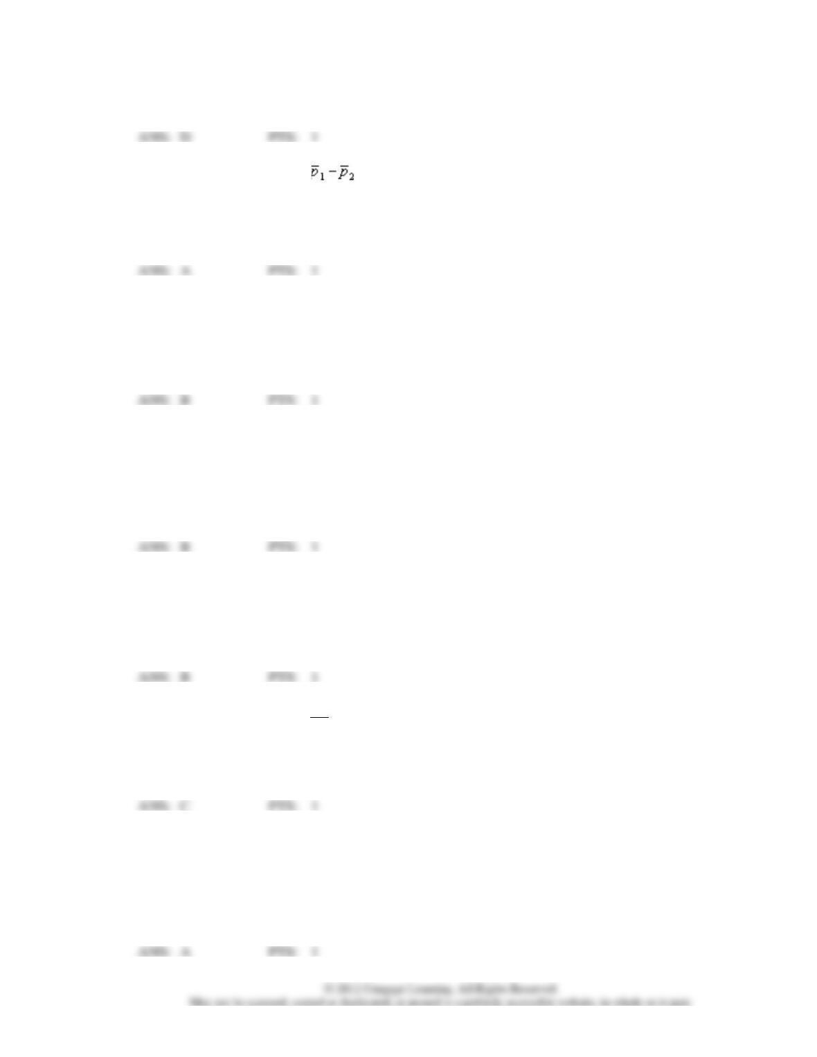
13. The sampling distribution of is approximated by a
a.
normal distribution
b.
t distribution with n1 + n2 degrees of freedom
c.
t distribution with n1 + n2 − 1 degrees of freedom
d.
t distribution with n1 + n2 + 2 degrees of freedom
14. If a hypothesis is rejected at 95% confidence,
a.
it must also be rejected at the 99% confidence
b.
it must also be rejected at the 90% confidence
c.
it will sometimes be rejected and sometimes not be rejected at the 90% confidence
d.
Not enough information is given to answer this question.
15. If the p-value is less than ,
a.
the alternative hypothesis is rejected
b.
the null hypothesis is rejected
c.
the null hypothesis will sometimes be rejected and sometimes not be rejected depending
on the sample size
d.
Not enough information is given to answer this question.
16. In a two-tailed hypothesis test the test statistic is determined to be z = -2.5. The p–value for this test
a.
is 0.0062
b.
is 0.0124
c.
is 0.4938
d.
cannot be determined, since the level of confidence is not given.
17. Which of the following does not need to be known in order to compute the p-value?
a.
knowledge of whether the test is one-tailed or two-tailed
b.
the value of the test statistic
c.
the level of significance
d.
All of the information provided is necessary.
18. A population where each element of the population is assigned to one and only one of several classes
or categories is a
a.
multinomial population
b.
Poisson population
c.
normal population
d.
None of these alternatives is correct.

19. The sampling distribution for a goodness of fit test is the
a.
Poisson distribution
b.
t distribution
c.
normal distribution
d.
chi-square distribution
20. A goodness of fit test is always conducted as a
a.
lower-tail test
b.
upper-tail test
c.
middle test
d.
None of these alternatives is correct.
21. An important application of the chi-square distribution is
a.
making inferences about a single population variance
b.
testing for goodness of fit
c.
testing for the independence of two variables
d.
All of these alternatives are correct.
22. The number of degrees of freedom for the appropriate chi-square distribution in a test of independence
is
a.
n − 1
b.
k − 1
c.
number of rows minus 1 times number of columns minus 1
d.
a chi-square distribution is not used
23. In order not to violate the requirements necessary to use the chi-square distribution, each expected
frequency in a goodness of fit test must be
a.
at least 5
b.
at least 10
c.
no more than 5
d.
less than 2
24. A statistical test conducted to determine whether to reject or not reject a hypothesized probability
distribution for a population is known as a
a.
contingency test
b.
probability test
c.
goodness of fit test
d.
None of these alternatives is correct.
25. The degrees of freedom for a contingency table with 12 rows and 12 columns is
a.
144
b.
121
c.
12
d.
120
26. The degrees of freedom for a contingency table with 6 rows and 3 columns is
a.
18
b.
6
c.
6
d.
10
27. The degrees of freedom for a contingency table with 10 rows and 11 columns is
a.
100
b.
110
c.
21
d.
90
Exhibit 11-1
The results of a recent poll on the preference of shoppers regarding two products are shown below.
Shoppers Favoring
Product
Shoppers Surveyed
This Product
A
800
560
B
900
612
28. Refer to Exhibit 11-1. The point estimate for the difference between the two population proportions in
favor of this product is
a.
52
b.
100
c.
0.44
d.
0.02
29. Refer to Exhibit 11-1. The standard error of is
a.
52
b.
0.044
c.
0.0225
d.
100
30. Refer to Exhibit 11-1. At 95% confidence, the margin of error is
a.
0.064
b.
0.044
c.
0.0225
d.
52
31. Refer to Exhibit 11-1. The 95% confidence interval estimate for the difference between the
populations favoring the products is
a.
-0.024 to 0.064
b.
0.6 to 0.7
c.
0.024 to 0.7
d.
0.02 to 0.3
Exhibit 11-2
An insurance company selected samples of clients under 18 years of age and over 18 and recorded the
number of accidents they had in the previous year. The results are shown below.
Under Age of 18
Over Age of 18
n1 = 500
n2 = 600
Number of accidents = 180
Number of accidents = 150
We are interested in determining if the accident proportions differ between the two age
groups.
32. Refer to Exhibit 11-2 and let pU represent the proportion under and pO the proportion over the age of
18. The null hypothesis is
a.
pU − pO 0
b.
pU − pO 0
c.
pU − pO 0
d.
pU − pO = 0
33. Refer to Exhibit 11-2. The pooled proportion is
a.
0.305
b.
0.300
c.
0.027
d.
0.450
34. Refer to Exhibit 11-2. The test statistic is
a.
0.96
b.
1.96
c.
2.96
d.
3.96
35. Refer to Exhibit 11-2. The p-value is
a.
less than 0.001
b.
more than 0.10
c.
0.0228
d.
0.3
Exhibit 11-3
The results of a recent poll on the preference of teenagers regarding the types of music they listen to
are shown below.
Music
Teenagers
Teenagers Favoring
Type
Surveyed
This Type
Pop
800
384
Rap
900
450
36. Refer to Exhibit 11-3. The point estimate for the difference between the proportions is
a.
-0.02
b.
0.048
c.
100
d.
66
37. Refer to Exhibit 11-3. The standard error of is
a.
0.48
b.
0.50
c.
0.03
d.
0.0243
38. Refer to Exhibit 11-3. The 95% confidence interval for the difference between the two proportions is
a.
384 to 450
b.
0.48 to 0.5
c.
0.028 to 0.068
d.
-0.068 to 0.028
Exhibit 11-4
When individuals in a sample of 150 were asked whether or not they supported capital punishment, the
following information was obtained.
Do you support
Number of
capital punishment?
individuals
Yes
40
No
60
No Opinion
50
We are interested in determining whether or not the opinions of the individuals (as to Yes, No, and No
Opinion) are uniformly distributed.
39. Refer to Exhibit 11-4. The expected frequency for each group is
a.
0.333
b.
0.50
c.
1/3
d.
50
40. Refer to Exhibit 11-4. The calculated value for the test statistic equals
a.
2
b.
-2
c.
20
d.
4
41. Refer to Exhibit 11-4. The number of degrees of freedom associated with this problem is
a.
150
b.
149
c.
2
d.
3
42. Refer to Exhibit 11-4. The p-value is
a.
larger than 0.1
b.
less than 0.1
c.
less than 0.05
d.
larger than 0.9
43. Refer to Exhibit 11-4. The conclusion of the test (at 95% confidence) is that the
a.
distribution is uniform
b.
distribution is not uniform
c.
test is inconclusive
d.
None of these alternatives is correct.
Exhibit 11-5
Last school year, the student body of a local university consisted of 30% freshmen, 24% sophomores,
26% juniors, and 20% seniors. A sample of 300 students taken from this year’s student body showed
the following number of students in each classification.
Freshmen
83
Sophomores
68
Juniors
85
Seniors
64
We are interested in determining whether or not there has been a significant change in the
classifications between the last school year and this school year.
44. Refer to Exhibit 11-5. The expected number of freshmen is
a.
83
b.
90
c.
30
d.
10
45. Refer to Exhibit 11-5. The expected frequency of seniors is
a.
60
b.
20%
c.
68
d.
64
46. Refer to Exhibit 11-5. The calculated value for the test statistic equals
a.
0.5444
b.
300
c.
1.6615
d.
6.6615
47. Refer to Exhibit 11-5. The p-value is
a.
less than .005
b.
between .025 and 0.05
c.
between .05 and 0.1
d.
greater than 0.1
48. Refer to Exhibit 11-5. At 95% confidence, the null hypothesis
a.
should not be rejected
b.
should be rejected
c.
was designed wrong
d.
None of these alternatives is correct.
Exhibit 11-6
In order to determine whether or not a particular medication was effective in curing the common cold,
one group of patients was given the medication, while another group received sugar pills. The results
of the study are shown below.
Patients Cured
Patients Not Cured
Received medication
70
10
Received sugar pills
20
50
We are interested in determining whether or not the medication was effective in curing the common
cold.
49. Refer to Exhibit 11-6. The expected frequency of those who received medication and were cured is
a.
70
b.
150
c.
28
d.
48

50. Refer to Exhibit 11-6. The test statistic is
a.
10.08
b.
54.02
c.
1.96
d.
1.645
51. Refer to Exhibit 11-6. The number of degrees of freedom associated with this problem is
a.
4
b.
149
c.
1
d.
3
52. Refer to Exhibit 11-6. The hypothesis is to be tested at the 5% level of significance. The critical value
from the table equals
a.
3.84
b.
7.81
c.
5.99
d.
9.34
53. Refer to Exhibit 11-6. The p-value is
a.
less than .005
b.
between .005 and .01
c.
between .01 and .025
d.
between .025 and .05
Exhibit 11-7
In the past, 35% of the students at ABC University were in the Business College, 35% of the students
were in the Liberal Arts College, and 30% of the students were in the Education College. To see
whether or not the proportions have changed, a sample of 300 students was taken. Ninety of the
sample students are in the Business College, 120 are in the Liberal Arts College, and 90 are in the
Education College.
54. Refer to Exhibit 11-7. This problem is an example of a
a.
normally distributed variable
b.
test for independence
c.
Poisson distributed variable
d.
multinomial population
55. Refer to Exhibit 11-7. The expected frequency for the Business College is
a.
0.3
b.
0.35
c.
90
d.
105
56. Refer to Exhibit 11-7. The calculated value for the test statistic equals
a.
0.01
b.
0.75
c.
4.29
d.
4.38
57. Refer to Exhibit 11-7. The hypothesis is to be tested at the 5% level of significance. The critical value
from the table equals
a.
1.645
b.
1.96
c.
5.991
d.
7.815
58. Refer to Exhibit 11-7. The p-value is
a.
greater than 0.1
b.
between 0.05 and 0.1
c.
between 0.025 and 0.05
d.
between 0.01 and .025
59. Refer to Exhibit 11-7. The conclusion of the test is that the
a.
proportions have changed significantly
b.
proportions have not changed significantly
c.
test is inconclusive
d.
None of these alternatives is correct.
Exhibit 11-8
The table below gives beverage preferences for random samples of teens and adults.
Teens
Adults
Total
Coffee
50
200
250
Tea
100
150
250
Soft Drink
200
200
400
Other
50
50
100
400
600
1,000
We are asked to test for independence between age (i.e., adult and teen) and drink preferences.
60. Refer to Exhibit 11-8. With a .05 level of significance, the critical value for the test is
a.
1.645
b.
7.815
c.
14.067
d.
15.507
61. Refer to Exhibit 11-8. The expected number of adults who prefer coffee is
a.
0.25
b.
0.33
c.
150
d.
200
62. Refer to Exhibit 11-8. The test statistic for this test of independence is
a.
0
b.
8.4
c.
62.5
d.
82.5
63. Refer to Exhibit 11-8. The p-value is
a.
between .1 and .05
b.
between .05 and .025
c.
between .025 and .01
d.
less than 0.005
64. If the chi-square test indicates that there is no difference between two proportions, this indicates that
a.
the two variables are correlated
b.
the two variables are independent
c.
the two variables are dependent
d.
there is a relationship between the two variables
65. When a category in a contingency table has an expected frequency of less than five,
a.
switch from a one-tailed test to a two-tailed test
b.
conclude that the two variables are independent
c.
double the expected frequency in every category
d.
combine two adjacent categories to obtain an expected frequency of five or more
66. All of the following tests follow a chi-square distribution except
a.
test of independence of two variables
b.
test for the difference between two proportions
c.
test for proportions of a multinomial population
d.
test for the difference between two means
67. The degrees of freedom for a chi-square test involving 5 proportions are
a.
3
b.
4
c.
5
d.
6
68. When conducting a good of fit test, the expected frequencies for the multinomial population are based
on the
a.
chi-square distribution
b.
normal distribution
c.
null hypothesis
d.
alternative hypothesis
PROBLEM
1. Babies weighing less than 5.5 pounds at birth are considered “low-birth-weight babies.” In the United
States, 7.6% of newborns are low-birth-weight babies. The following information was accumulated
from samples of new births taken from two counties.
Hamilton
Shelby
Sample size
150
200
Number of “low-birth-weight babies
18
22
a.
Develop a 95% confidence interval estimate for the difference between the proportions of
low-weight babies in the two counties.
b.
Is there conclusive evidence that one of the proportions is significantly more than the other?
If yes, which county? Explain, using the results of Part a. Do not perform any test.
-.0577 to .0777
b.
Since the range of the interval is from negative to positive, there is no indication that one
proportion is significantly different (at 95% confidence) from the other.
2. Of 200 UTC seniors surveyed, 60 were planning on attending Graduate School. At UTK, 400 seniors
were surveyed; and 100 indicated that they were planning to attend Graduate School.
a.
Determine a 95% confidence interval estimate for the difference between the proportions of
seniors at the two universities that were planning to attend Graduate School.
b.
Is there conclusive evidence to prove that the proportion of students from UTC who plan to go
to Graduate School is significantly more than those from UTK? Explain.
-0.026 to 0.126
b.
No, the range of the interval is from a negative to a positive value.
3. Among a sample of 50 MDs (medical doctors) in the city of Memphis, Tennessee, 10 indicated they
make house calls; while among a sample of 100 MDs in Atlanta, Georgia, 18 said they make house
calls. Determine a 95% interval estimate for the difference between the proportions of doctors who
make house calls in the two cities.
4. Of 150 Chattanooga residents surveyed, 60 indicated that they participated in a recycling program. In
Knoxville, 120 residents were surveyed and 36 claimed to recycle.
a.
Determine a 95% confidence interval estimate for the difference between the proportions of
residents recycling in the two cities.
b.
From your answer in Part a, is there sufficient evidence to conclude that there is a significant
difference in the proportion of residents participating in a recycling program?
-0.0134 to 0.2134
b.
No, because the interval for the proportions ranges from a negative to a positive value.
5. During the primary elections of 2008, candidate A showed the following pre-election voter support in
Tennessee and Mississippi.
Voters Favoring
Voters Surveyed
Candidate A
Tennessee
500
295
Mississippi
700
357
a.
Develop a 95% confidence interval estimate for the difference between the proportion of
voters favoring candidate A in the two states.
b.
Is there conclusive evidence that one of the two states had a larger proportion of voters’
support? If yes, which state? Explain.
0.023 to 0.137
b.
Yes, the range of interval is from positive to positive, indicating Tennessee had the larger
support.
6. In a sample of 40 Democrats, 6 opposed the President’s foreign policy, while of 50 Republicans, 8
were opposed to his policy. Determine a 90% confidence interval estimate for the difference between
the proportions of the opinions of the individuals in the two parties.
7. The results of a recent poll on the preference of voters regarding the presidential candidates are shown
below.
Voters Favoring
Voters Surveyed
This Candidate
Candidate A
200
150
Candidate B
300
195
a.
Develop a 90% confidence interval estimate for the difference between the proportions of
voters favoring each candidate.
b.
Does your confidence interval provide conclusive evidence that one of the candidates is
favored more? Explain.
0.032 to 0.168
b.
Yes, the range of interval is from positive to positive, indicating Candidate A had the larger
support.
8. In a random sample of 200 Republicans, 160 opposed the new tax laws. While in a sample of 120
Democrats, 84 opposed the new tax laws. Determine a 95% confidence interval estimate for the
difference between the proportions of Republicans and Democrats opposed to this new law.
9. From production line A, a sample of 500 items is selected at random; and it is determined that 30 items
are defective. In a sample of 300 items from production process B (which produces identical items to
line A), there are 12 defective items. Determine a 95% confidence interval estimate for the difference
between the proportions of defectives in the two lines.
10. A poll was taken this year asking college students if they considered themselves overweight. A similar
poll was taken five ago. Results are summarized below. Has the proportion increased significantly?
Let = 0.05.
Number Considered
Sample Size
Themselves Overweight
Current Sample (c)
300
150
Previous Sample (p)
275
121
11. Of 300 female registered voters surveyed, 120 indicated they were planning to vote for the incumbent
president; while of 400 male registered voters, 140 indicated they were planning to vote for the
incumbent president.
a.
Compute the test statistic.
b.
At alpha = .05, test to see if there is a significant difference between the proportions of females
and males who plan to vote for the incumbent president. (Use the p-value approach.)
12. During the recent primary elections, the democratic presidential candidate showed the following pre–
election voter support in Alabama and Mississippi.
Voters Favoring the
State
Voters Surveyed
Democratic Candidate
Alabama
800
440
Mississippi
600
360
a.
We want to determine whether or not the proportions of voters favoring the Democratic
candidate were the same in both states. Provide the hypotheses.
b.
Compute the test statistic.
c.
Determine the p-value; and at 95% confidence, test the above hypotheses.
13. A comparative study of organic and conventionally grown produce checked for the presence of E. coli.
Results are summarized below. Is there a significant difference in the proportion of E. Coli in organic
versus conventionally grown produce? Test at = 0.10.
Sample Size
E. Coli Prevalence
Organic
200
3
Conventional
500
20
14. In a sample of 100 Republicans, 60 favored the President’s anti-drug program. While in a sample of
150 Democrats, 84 favored his program. At 95% confidence, test to see if there is a significant
difference in the proportions of the Democrats and the Republicans who favored the President’s anti-
drug program.
15. The office of records at a university has stated that the proportion of incoming female students who
major in business has increased. A sample of female students taken several years ago is compared with
a sample of female students this year. Results are summarized below. Has the proportion increased
significantly? Test at alpha = .10.
Sample Size
No. Majoring in Business
Previous Sample (p)
250
75
Current Sample (c)
300
69
16. The reliability of two types of machines used in the same manufacturing process is to be tested. The
first machine failed to operate correctly in 90 out of 300 trials while the second type failed to operate
correctly in 50 out of 250 trials.
a.
Give a point estimate for the difference between the population proportions of these machines.
b.
Calculate the pooled estimate of the population proportion.
c.
Carry out a hypothesis test to check whether there is a statistically significant difference in the
reliability for the two types of machines using a .10 level of significance.
a.
0.10
b.
0.2545
test statistic z = 2.68, p-value = 0.0074, reject H0
17. The results of a recent poll on the preference of voters regarding presidential candidates are shown
below.
Voters Favoring
Candidate
Voters Surveyed
This Candidate
A
400
192
B
450
225
At 95% confidence, test to determine whether or not there is a significant difference between the
preferences for the two candidates.
18. A school administrator believes that there is no difference between student dropout rate for schools
located in rural areas and schools located in urban areas. A random sample of 100 schools in the rural
areas was taken. The student dropout rate of the schools in the sample was 27%. A random sample of
80 schools in the urban areas had a dropout rate of 20%.
a.
Give a point estimate for the difference between the population proportions for the two
districts.
b.
Give a point estimate of the standard deviation for the difference between the population
proportions.
c.
Compute the test statistic for testing the administrator’s belief.
d.
At 95% confidence using the p-value approach, test the administrator’s belief.
0.07
b.
0.064
Test statistic z = 1.09
19. Before the start of the Winter Olympics, it was expected that the percentages of medals awarded to the
top contenders to be as follows.
Percentages
United States
25%
Germany
22%
Norway
18%
Austria
14%
Russia
11%
France
10%
Midway through the Olympics, of the 120 medals awarded, the following distribution was observed.
Number of Medals
United States
33
Germany
36
Norway
18
Austria
15
Russia
12
France
6
We want to test to see if there is a significant difference between the expected and actual awards given.
a.
Compute the test statistic.
b.
Using the p-value approach, test to see if there is a significant difference between the expected
and the actual values. Let = .05.
c.
At 95% confidence, test for a significant difference using the critical value approach.
b.
20. A medical journal reported the following frequencies of deaths due to cardiac arrest for each day of the
week.
Day
Cardiac Deaths
Monday
40
Tuesday
17
Wednesday
16
Thursday
29
Friday
15
Saturday
20
Sunday
17
We want to determine whether the number of deaths is uniform over the week.
a.
Compute the test statistic.
b.
Using the p-value approach at 95% confidence, test for the uniformity of death over the week.
c.
Using the critical value approach, perform the test for uniformity.
b.
21. Before the presidential debates, it was expected that the percentages of registered voters in favor of
various candidates would be as follows.
Percentage
Democrats
48%
Republicans
38%
Independents
4%
Undecided
10%