
Chapter 11 – Simulation Models
1. Which of the following is typically not an application of simulation models?
a.
Operations models
b.
Financial models
c.
Marketing models
d.
Logistics models
d
1
2. Which of the following is the most likely characteristic of a distribution that is to be used to develop a simulation model
for estimating the time until failure of a product in a simulation model?
a.
Unbounded
b.
Left skewed
c.
Normal
d.
Uniform
b
1
3. Which of the following functions is not an @RISK statistical function?
a.
RISKMIN
b.
RISKMAX
c.
RISKPERCENTILE
d.
RISKSIMTABLE
d
1
4. Which of the following @RISK functions can be used to find the probability of a particular value in an output
distribution?
a.
RISKMIN
b.
RISKMAX
c.
RISKPERCENTILE
d.
RISKTARGET
d
1
5. Value at risk (VAR) is an indicator of:
a.
how much to bid for a project
b.
the expected amount of loss for a project
c.
what is nearly the worst possible outcome for a project
d.
the required amount of investment required for a project
c
1
6. The value at risk (VAR) is typically defined as the:
a.
5th percentile of NPV distribution
b.
10th percentile of NPV distribution

Chapter 11 – Simulation Models
c.
90th percentile of NPV distribution
d.
95th percentile of NPV distribution
a
1
7. Suppose we compare the difference between the NPV of a financial model in which the means are entered for all input
random variables and the NPV of a financial model in which the most likely values are entered for all input random
variables. If we see a large difference between the NPV’s, this illustrates:
a.
the value at risk (VAR)
b.
the effect of randomness
c.
the flaw of averages
d.
the bias of the analyst
c
1
8. In cash flow models, we are typically interested in investigating:
a.
the value at risk (VAR)
b.
the net present value (NPV)
c.
the amount of loans required to maintain a minimum cash balance
d.
the interest on loans taken out by a firm
c
1
9. A key input variable in many marketing models of customer loyalty is the:
a.
Mean profit per customer
b.
Number of customers
c.
Churn rate
d.
Time horizon
c
1
10. The main issue in marketing and sales models is:
a.
the amount invested in marketing
b.
the timing of marketing
c.
the profit from sales
d.
the timing of sales
d
1
11. In bidding models, the simulation output variable is the number of competitors who will bid.
a.
True
b.
False
False
1

12. In warranty cost models, the key input random variable is product lifetime.
a.
True
b.
False
True
1
13. A common distribution for modeling product lifetimes is the normal distribution
a.
True
b.
False
False
1
14. The RISKSIMTABLE function is used to summarize the results of a single simulation of product lifetime.
a.
True
b.
False
False
1
15. RISKTARGET is a function that allows us to determine the cumulative probability of a particular value in an output
distribution, such as the probability of meeting a due date in manufacturing.
a.
True
b.
False
True
1
16. In financial simulation models, we are typically more interested in the expected NPV of a project than in the extremes
of the outcomes.
a.
True
b.
False
False
1
17. A tornado chart lets us see which random input has the most effect on a specified output in a financial model.
a.
True
b.
False
True
1
18. A marketing simulation model can be used to determine the expected profit under uncertain customer loyalty, but an
optimization model must be used to determine the optimal amount to spend on increasing customer loyalty.
a.
True
b.
False
False
1
19. In marketing and sales models, the primary issue is the uncertain amount of sales that can be obtained, given an
Chapter 11 – Simulation Models
assumed timing.
a.
True
b.
False
False
1
20. A @RISK output range allows us to obtain a summary chart that shows the entire simulated range at once.
a.
True
b.
False
True
1
Exhibit 11-1
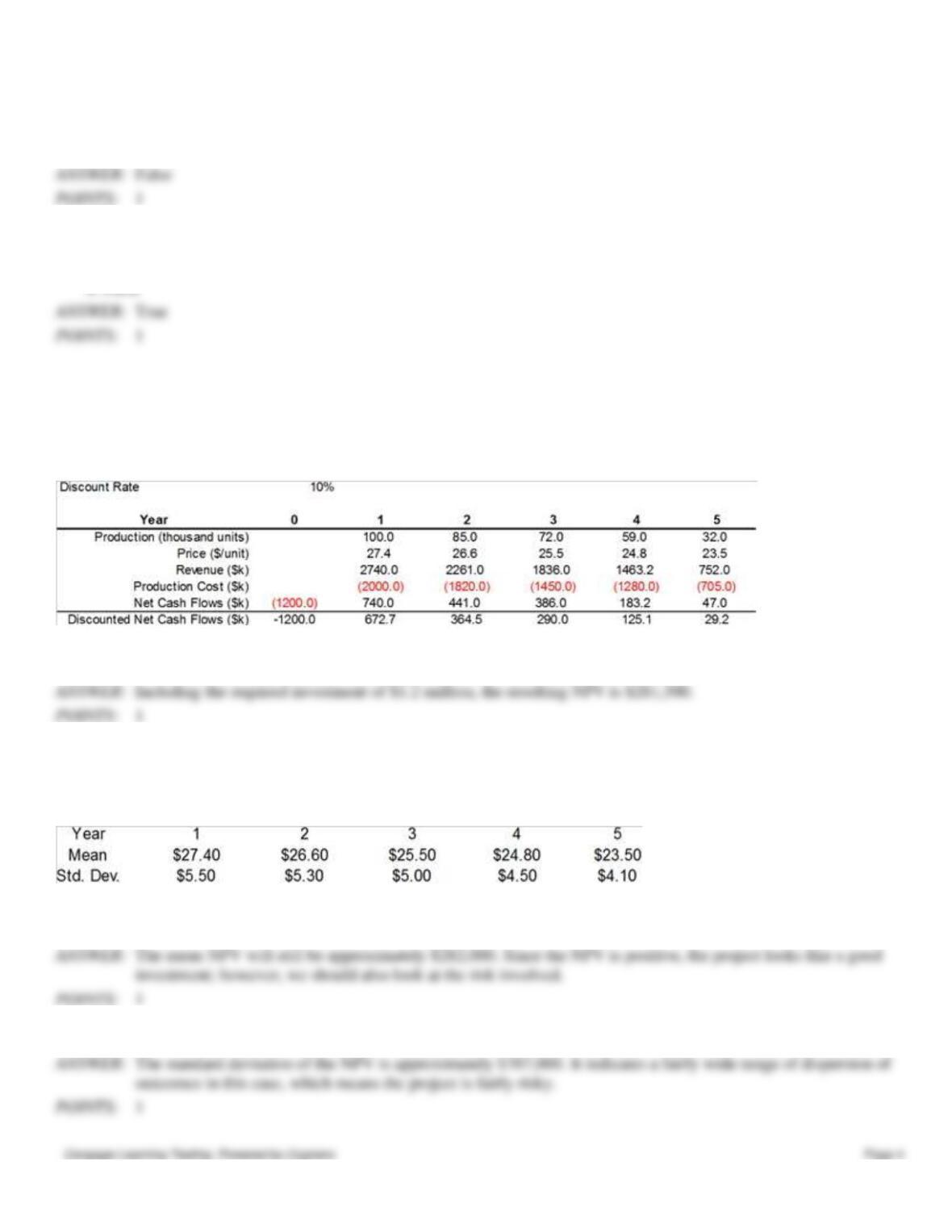
A company is considering investing $1.2M in a facility to manufacture a new product. The product will have a five year
life, after which the facility will be shut down. A pro forma cash flow sheet for this project, with forecasted production
levels, unit prices, and production costs, is shown below:
21. [Part 1] Refer to Exhibit 11–1. What is the deterministic next present value (NPV) of the project, including the
required investment, assuming a 10% discount rate?
1
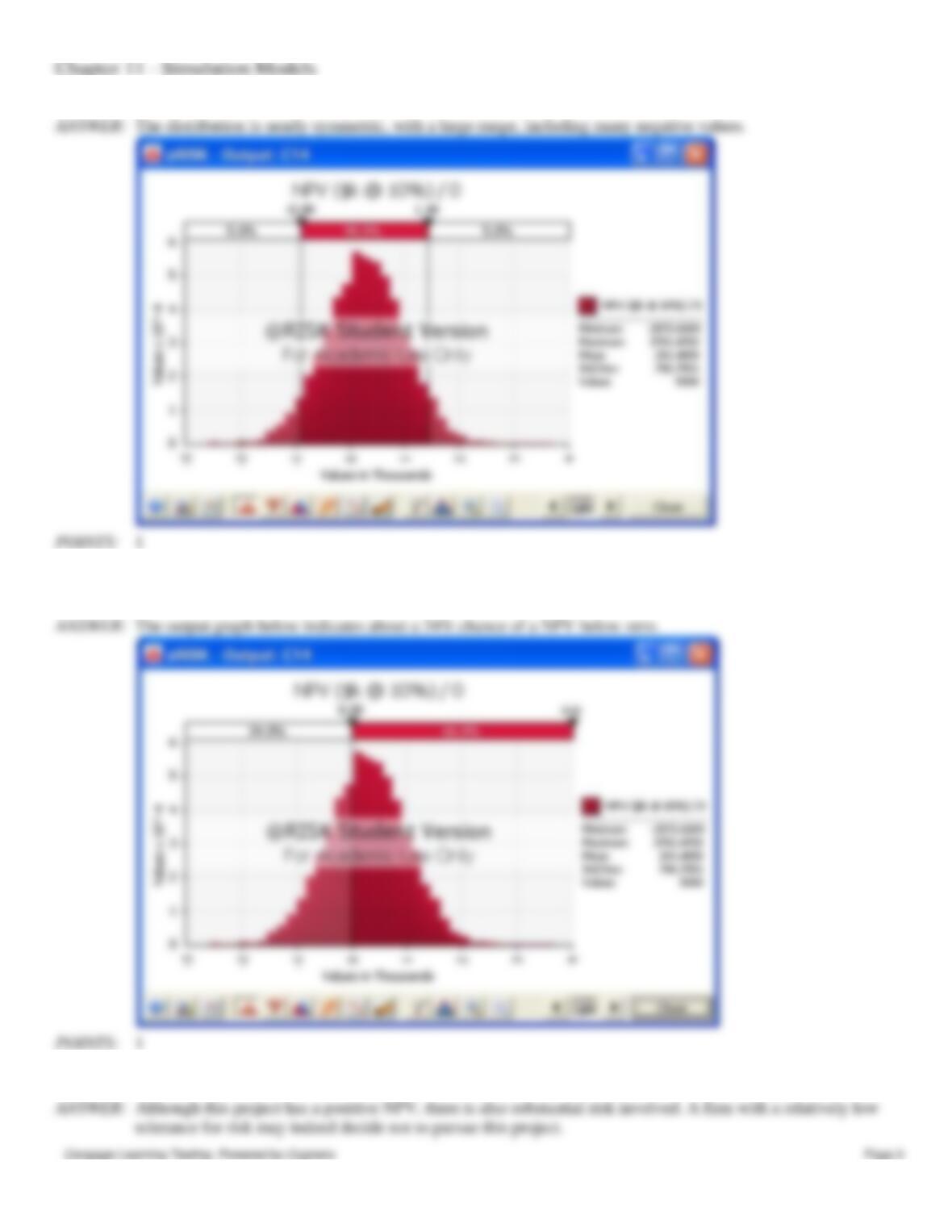
22. [Part 2] Refer to Exhibit 11–1. Suppose that the forecasted price levels shown in the pro forma cash flow sheet are not
deterministic, but rather are expected to fluctuate due to market forces. The prices are expected to be normally distributed
in each year, with the following means and standard deviations:
Using the appropriate @RISK functions in the pro forma, what is the expected NPV? Would you recommend investing in
this project? Explain.
1
23. [Part 3] Refer to Exhibit 11–1. What is the standard deviation of the NPV? What does it indicate?
1
24. [Part 4] Refer to Exhibit 11–1. What does the distribution of the project NPV look like?
25. [Part 5] Refer to Exhibit 11–1. What are the chances the firm could lose money on this project, given the price
uncertainty?
26. [Part 6] Refer to Exhibit 11–1. Given your answers to Parts 1 through 5, would you invest in this project?
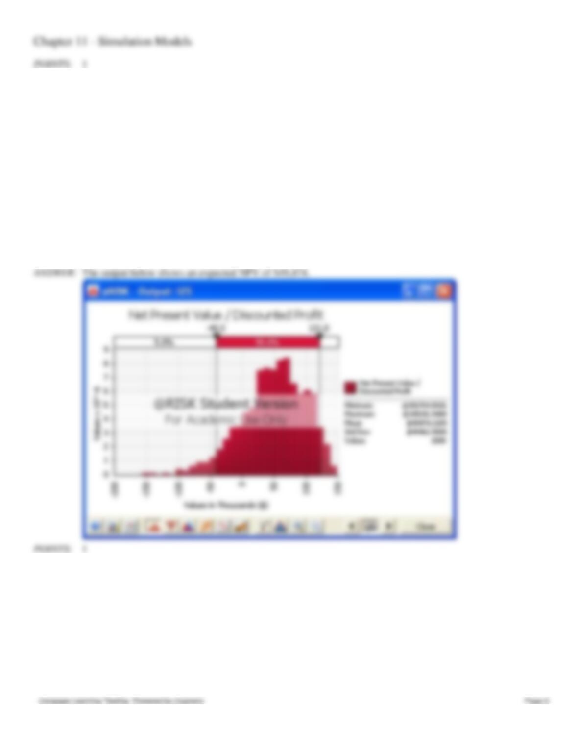
Exhibit 11-2
Suppose we want to choose capacity for a plant that will produce a new drug. In particular, we want to choose the
capacity that maximizes discounted expected profit over the next 10 years. Assume all cash flows occur at the end of the
year. We have the following information:
∙
Demand for the drug is expected to be normally distributed ˜ Normal (50,000, 12,000).
Demand each year is an independent event.
∙
A unit of capacity costs $16 to build in year 1.
∙
The number of units produced will equal the demand, up to capacity limits.
∙
The revenue per unit is $3.70 and the cost per unit is $0.20 (variable cost).
∙
The maintenance cost per unit of capacity is $0.40 (fixed cost).
∙
The discount rate is 10%.
27. [Part 1] Refer to Exhibit 11–2. Perform a simulation assuming the plant will be designed to meet the expected
demand. What is the net present value (NPV) in that case?
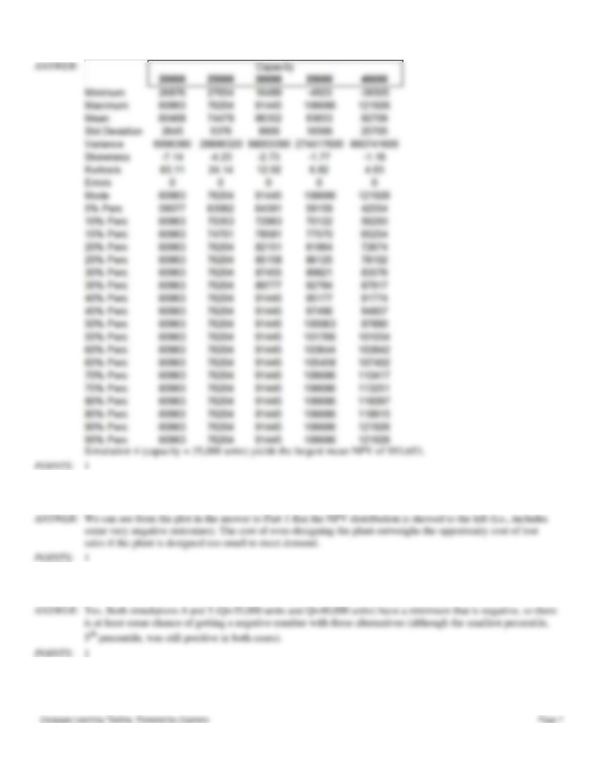
28. [Part 2] Refer to Exhibit 11–2. Use a RISKSIMTABLE to with the following values for capacity: 20,000, 25,000,
30,000, 35,000, 40,000. Which of these capacities produces the largest expected NPV?
Chapter 11 – Simulation Models
29. [Part 3] Refer to Exhibit 11–2. Briefly explain why designing the plant for the expected capacity is clearly not the
optimal solution.
30. [Part 4] Refer to Exhibit 11–2. Are there any simulations which indicated there was a chance of getting negative
NPV? Briefly explain in one sentence.