Name:
Class:
Date:
chapter 11
Indicate whether the statement is true or false.
1. In order to estimate with 90% confidence a particular value of Y for a given value of X in a simple linear regression
problem, a random sample of 20 observations is taken. The appropriate t-value that would be used is 1.734.
a.
True
b.
False
2. Multicollinearity is a situation in which two or more of the explanatory variables are highly correlated with each other.
a.
True
b.
False
3. In multiple regression, the problem of multicollinearity affects the t–tests of the individual coefficients as well as the F–
test in the analysis of variance for regression, since the F-test combines these t-tests into a single test.
a.
True
b.
False
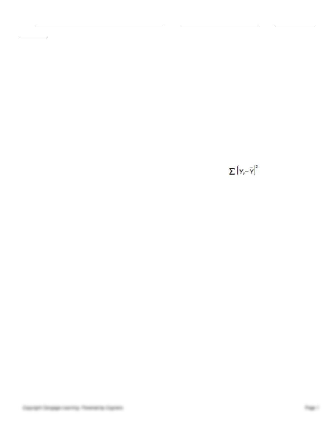
4. In regression analysis, the total variation in the dependent variable Y, measured by and referred to as SST,
can be decomposed into two parts: the explained variation, measured by SSR, and the unexplained variation, measured
by SSE.
a.
True
b.
False
5. Multiple regression represents an improvement over simple regression because it allows any number of response
variables to be included in the analysis.
a.
True
b.
False
6. In a multiple regression problem involving 30 observations and four explanatory variables, SST = 800 and SSE = 240.
The value of the F-statistic for testing the significance of this model is 14.583.
a.
True
b.
False
7. When there is a group of explanatory variables that are in some sense logically related, all of them must be included in
the regression equation.
a.
True
b.
False
8. One method of dealing with heteroscedasticity is to try a logarithmic transformation of the data.
a.
True
b.
False
9. Heteroscedasticity means that the variability of Y values is larger for some X values
than for others.
a.
True
b.
False
Name:
Class:
Date:
chapter 11
10. A multiple regression model involves 40 observations and 4 explanatory variables produces SST = 1000 and SSR =
804. The value of MSE is 5.6.
a.
True
b.
False
11. In time series data, errors are often not probabilistically independent.
a.
True
b.
False
12. If exact multicollinearlity exists, that means that there is redundancy in the data.
a.
True
b.
False
13. In a simple linear regression problem, if the standard error of estimate = 15 and n = 8, then the sum of squares for
error, SSE, is 1,350.
a.
True
b.
False
14. In order to test the significance of a multiple regression model involving 4 explanatory variables and 40 observations,
the numerator and denominator degrees of freedom for the critical value of F are 4 and 35, respectively.
a.
True
b.
False
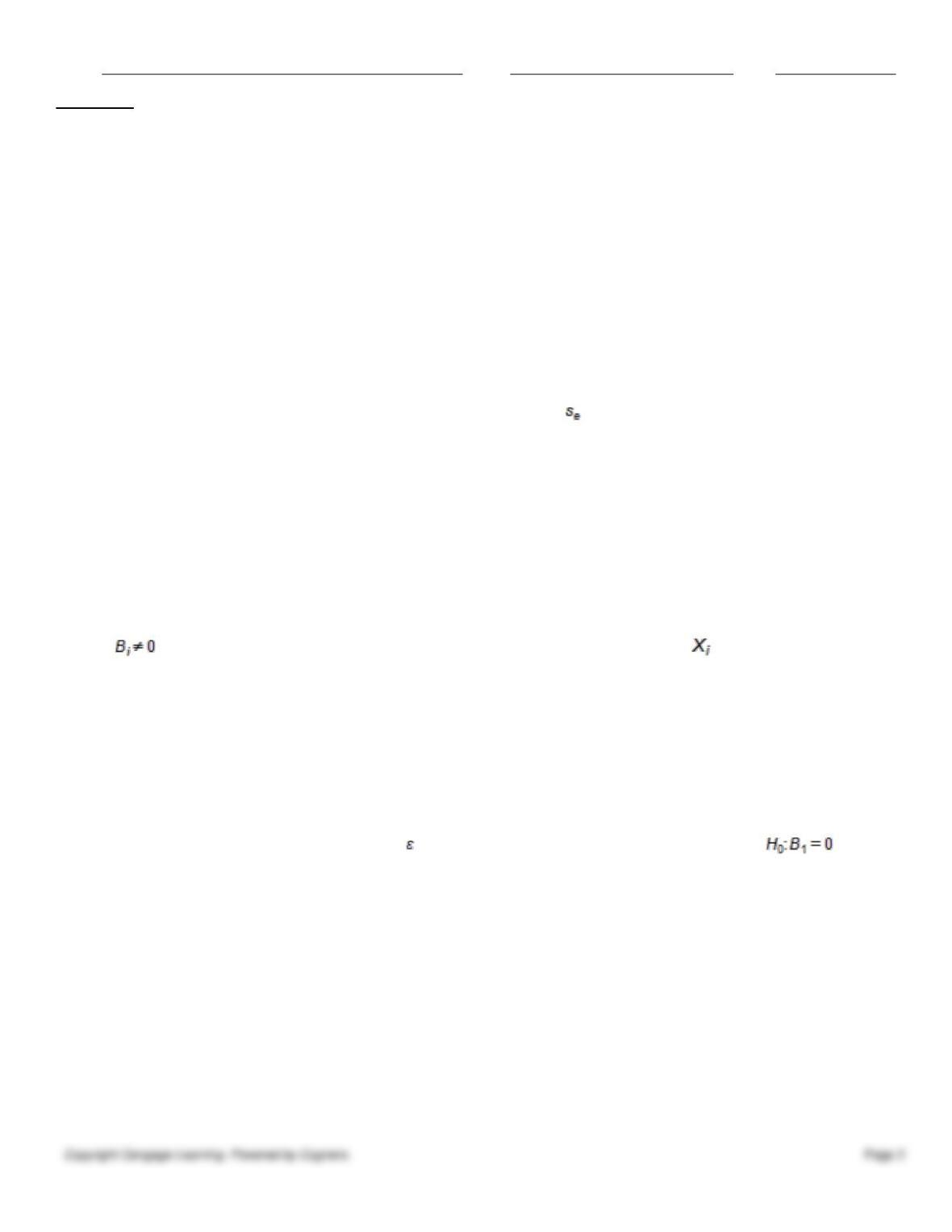
15. In multiple regression with k explanatory variables, the t-tests of the individual coefficients allows us to determine
whether (for i = 1, 2, …., k), which tells us whether a linear relationship exists between and Y.
a.
True
b.
False
16. Suppose that one equation has 3 explanatory variables and an F-ratio of 49. Another equation has 5 explanatory
variables and an F-ratio of 38. The first equation will always be considered a better model.
a.
True
b.
False
17. In simple linear regression, if the error variable is normally distributed, the test statistic for testing is t-
distributed with n – 2 degrees of freedom.
a.
True
b.
False
18. One of the potential characteristics of an outlier is that the value of the dependent variable is much larger or smaller
than predicted by the regression line.
a.
True
b.
False
19. In a multiple regression analysis involving 4 explanatory variables and 40 data points, the degrees of freedom
associated with the sum of squared errors, SSE, is 35.
a.
True
b.
False
Name:
Class:
Date:
chapter 11
20. In multiple regression, if there is multicollinearity between independent variables, the t-tests of the individual
coefficients may indicate that some variables are not linearly related to the dependent variable, when in fact they are.
a.
True
b.
False
21. A confidence interval constructed around a point prediction from a regression model is called a prediction interval,
because the actual point being estimated is not a population parameter
a.
True
b.
False
22. The Durbin-Watson statistic can be used to measure of autocorrelation.
a.
True
b.
False
23. A backward procedure is a type of equation building procedure that begins with all potential explanatory variables in
the regression equation and deletes them two at a time until further deletion would reduce the percentage of variation
explained to a value less than 0.50.
a.
True
b.
False
24. One method of diagnosing heteroscedasticity is to plot the residuals against the predicted values of Y, then look for a
change in the spread of the plotted values.
a.
True
b.
False
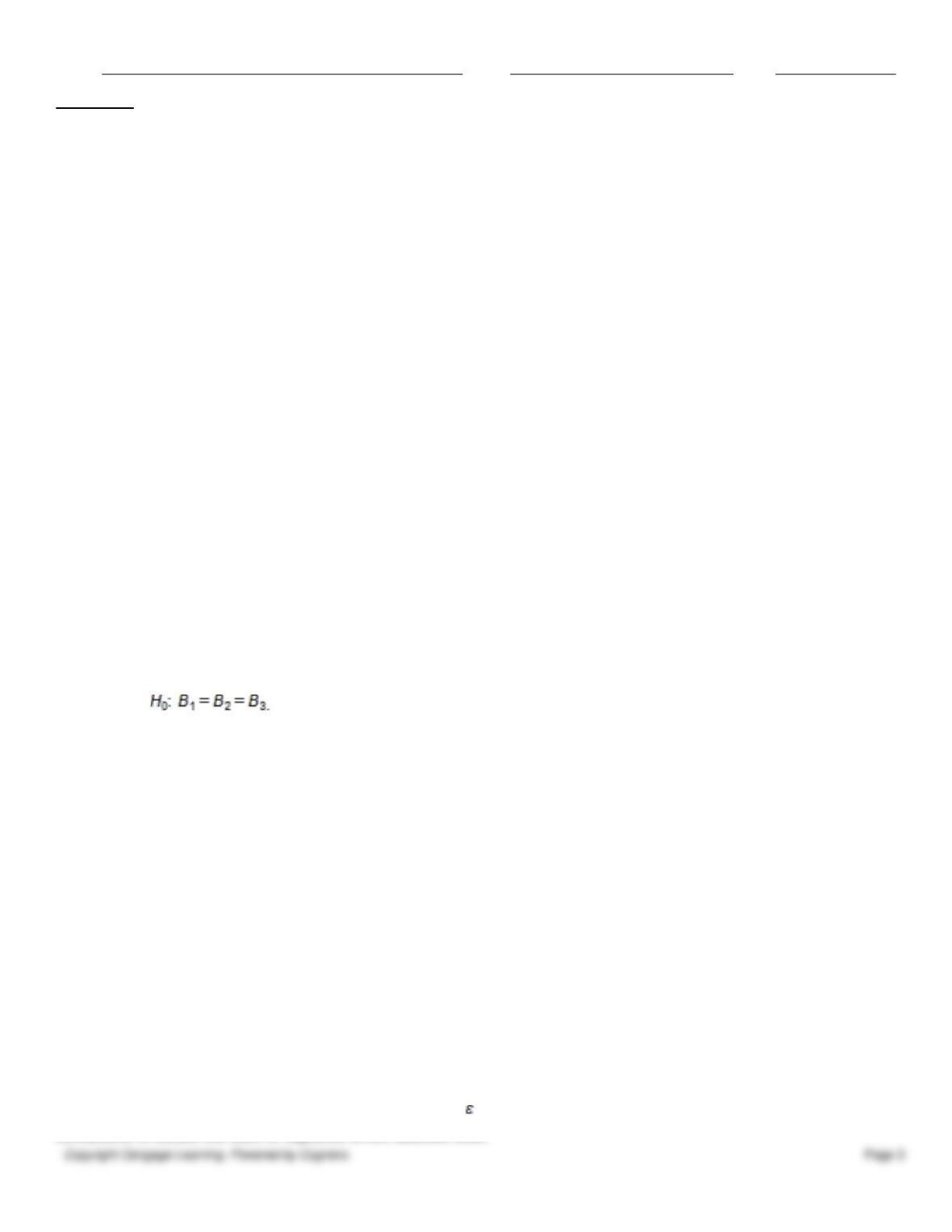
25. In testing the overall fit of a multiple regression model in which there are three explanatory variables, the null
hypothesis is .
a.
True
b.
False
26. In regression analysis, the unexplained part of the total variation in the response variable Y is referred to as sum of
squares due to regression, SSR.
a.
True
b.
False
27. In regression analysis, homoscedasticity refers to constant error variance.
a.
True
b.
False
28. In multiple regressions, a large value of the test statistic F indicates that most of the variation in Y is unexplained by
the regression equation and that the model is useless. A small value of F indicates that most of the variation in Y is
explained by the regression equation and that the model is useful.
a.
True
b.
False
29. The residuals are observations of the error variable . Consequently, the minimized sum of squared
deviations is called the sum of squared error, labeled SSE.

Name:
Class:
Date:
chapter 11
a.
True
b.
False
30. The value of the sum of squares due to regression, SSR, can never be larger than the value of the sum of squares
total, SST.
a.
True
b.
False
31. In a simple linear regression model, testing whether the slope of the population regression line could be zero is the
same as testing whether or not the linear relationship between the response variable Y and the explanatory variable X is
significant.
a.
True
b.
False
32. The assumptions of regression are: 1) there is a population regression line, 2) the dependent variable is normally
distributed, 3) the standard deviation of the response variable remains constant as the explanatory variables increase,
and 4) the errors are probabilistically independent.
a.
True
b.
False
33. Homoscedasticity means that the variability of Y values is the same for all X values.
a.
True
b.
False
34. A forward procedure is a type of equation building procedure that begins with only one explanatory variable in the
regression equation and successively adds one variable at a time until no remaining variables make a significant
contribution.
a.
True
b.
False
Indicate the answer choice that best completes the statement or answers the question.
35. Which of the following is not one of the guidelines for including/excluding variables in a regression equation?
a.
Look at t-value and associated p-value
b.
Check whether t-value is less than or greater than 1.0
c.
Variables are logically related to one another
d.
Use economic or physical theory to make decision
e.
All of these options are guidelines
36. When determining whether to include or exclude a variable in regression analysis, if the p-value associated with the
variable’s t-value is above some accepted significance value, such as 0.05, then the variable:
a.
is a candidate for inclusion
b.
is a candidate for exclusion
c.
is redundant
d.
not fit the guidelines of parsimony
37. Suppose you run a regression of a person’s height on his/her right and left foot sizes, and you suspect that there may
Name:
Class:
Date:
chapter 11
be multicollinearity between the foot sizes. What types of problems might you see if your suspicions are true?
a.
“Wrong” values for the coefficients for the left and right foot size
b.
Large p-values for the coefficients for the left and right foot size
c.
Small t-values for the coefficients for the left and right foot size
d.
All of these options
38. The can be used to test for autocorrelation.
a.
regression coefficient
b.
correlation coefficient
c.
Durbin-Watson statistic
d.
F-test or t-test
39. A scatterplot that exhibits a “fan” shape (the variation of Y increases as X increases) is an example of:
a.
homoscedasticity
b.
heteroscedasticity
c.
autocorrelation
d.
multicollinearity
40. Which of the following would be considered a definition of an outlier?
a.
An extreme value for one or more variables
b.
A value whose residual is abnormally large in magnitude
c.
Values for individual explanatory variables that fall outside the general pattern of the other observations
d.
All of these options
41. The value k in the number of degrees of freedom, n-k-1, for the sampling distribution of the regression coefficients
represents:
a.
the sample size
b.
the population size
c.
the number of coefficients in the regression equation, including the constant
d.
the number of independent variables included in the equation
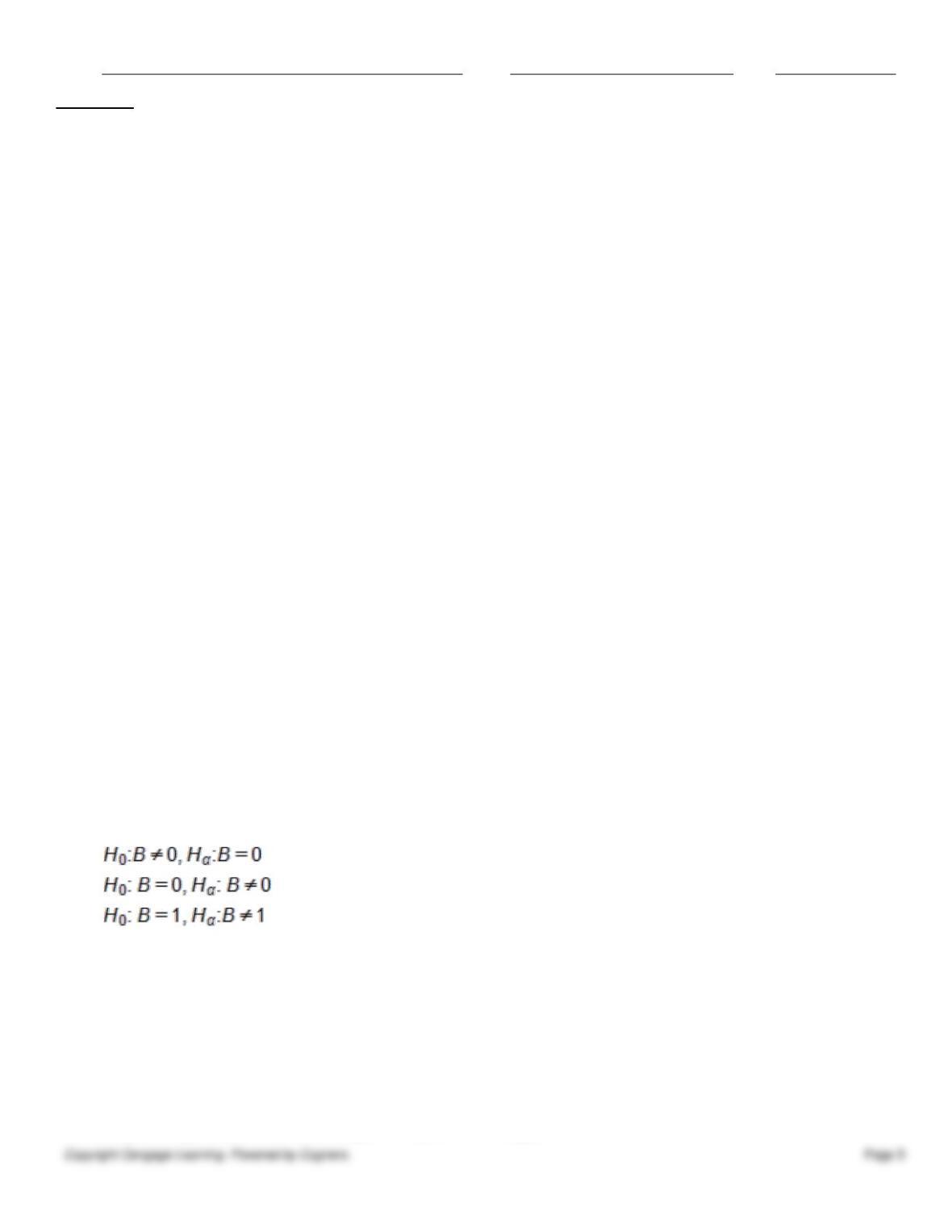
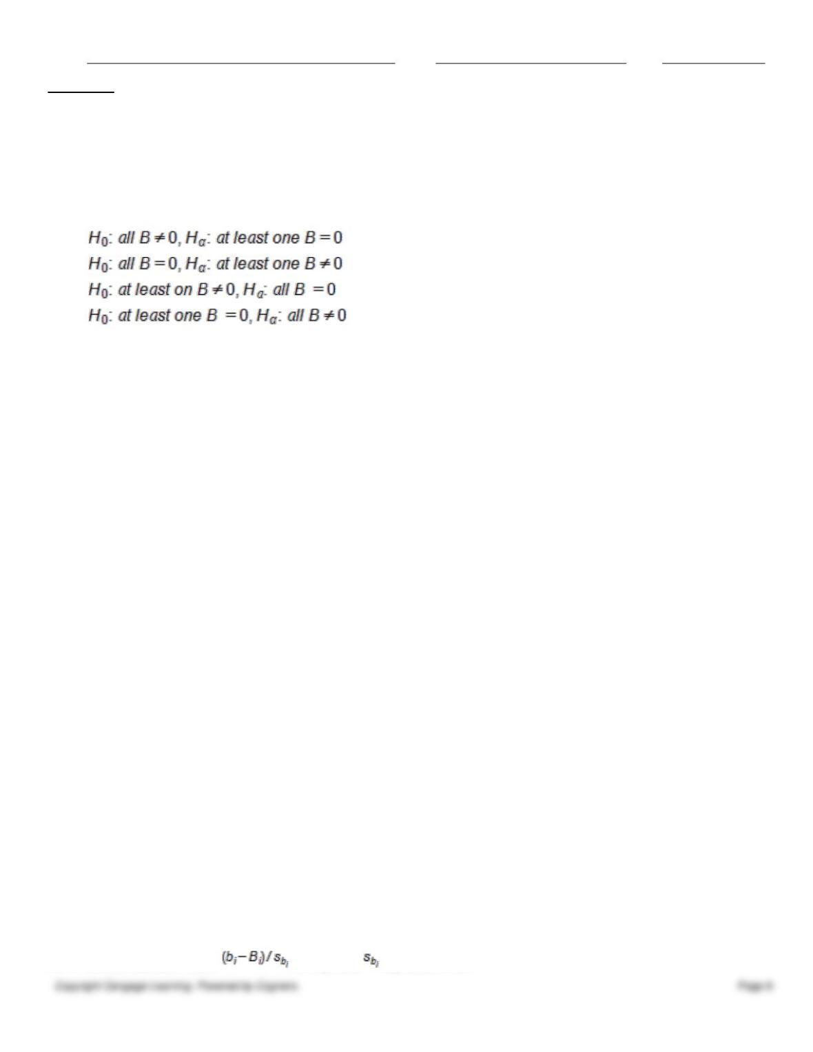
42. The appropriate hypothesis test for a regression coefficient is:
a.
b.
c.
d.
None of these options
43. The ANOVA table splits the total variation into two parts. They are the
a.
acceptable and unacceptable variation
b.
adequate and inadequate variation
c.
resolved and unresolved variation
d.
explained and unexplained variation
44. The objective typically used in the tree types of equation-building procedures are to:
Name:
Class:
Date:
chapter 11
a.
find the equation with a small se
b.
find the equation with a large R2
c.
find the equation with a small se and a large R2
d.
find the equation with the largest F-statistic
45. The appropriate hypothesis test for an ANOVA test is:
a.
b.
c.
d.
46. The error term represents the vertical distance from any point to the
a.
estimated regression line
b.
population regression line
c.
value of the Y’s
d.
mean value of the X’s
47. Determining which variables to include in regression analysis by estimating a series of regression equations by
successively adding or deleting variables according to prescribed rules is referred to as:
a.
elimination regression
b.
forward regression
c.
backward regression
d.
stepwise regression
48. Time series data often exhibits which of the following characteristics?
a.
homoscedasticity
b.
heteroscedasticity
c.
autocorrelation
d.
multicollinearity
49. In regression analysis, extrapolation is performed when you:
a.
attempt to predict beyond the limits of the sample
b.
have to estimate some of the explanatory variable values
c.
have to use a lag variable as an explanatory variable in the model
d.
don’t have observations for every period in the sample
50. Which of the following is the relevant sampling distribution for regression coefficients?
a.
Normal distribution
b.
t-distribution with n-1 degrees of freedom
c.
t-distribution with n-1-k degrees of freedom
d.
F-distribution with n-1-k degrees of freedom
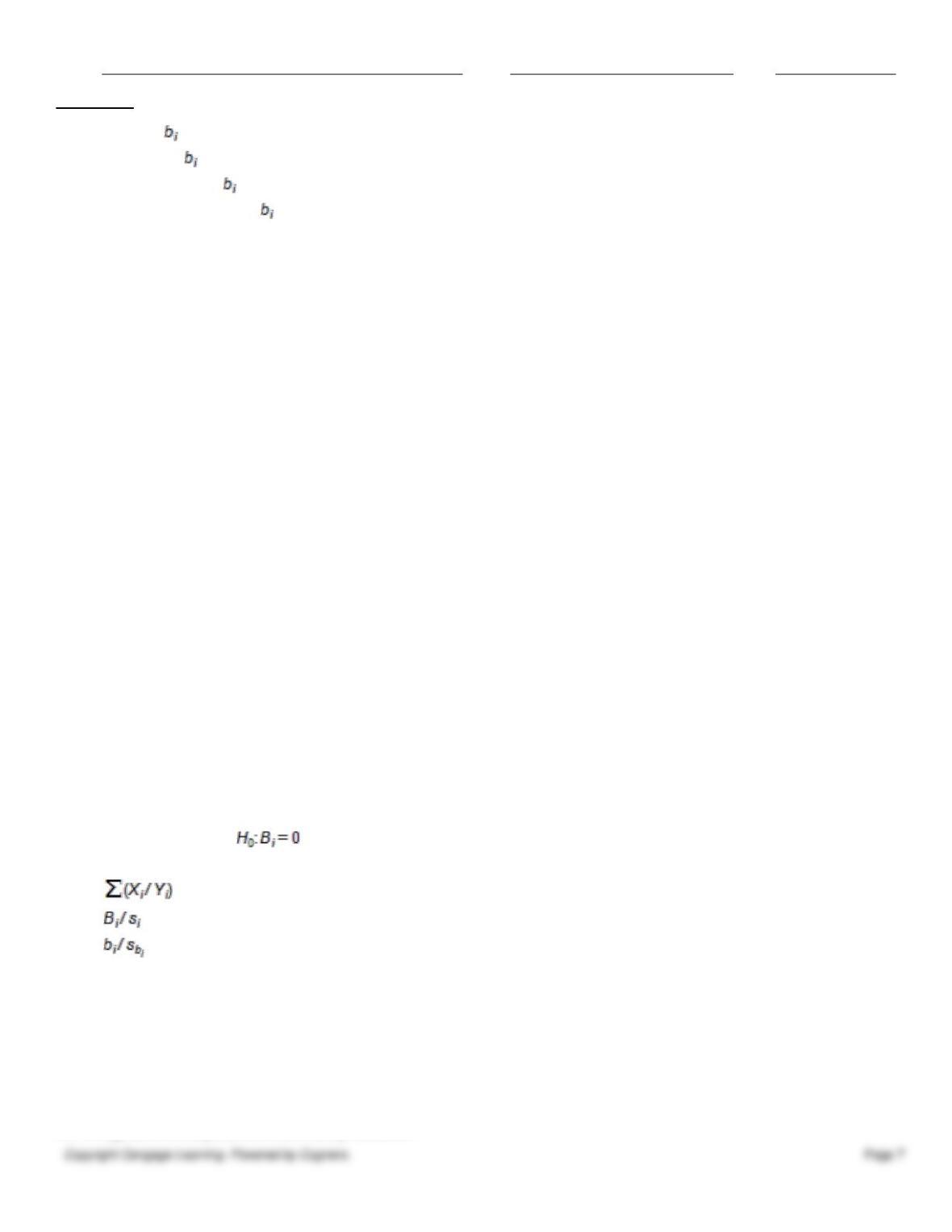
51. In the standardized value , the symbol represents the:
Name:
Class:
Date:
chapter 11
a.
mean of
b.
variance of
c.
standard error of
d.
degrees of freedom of
52. A point that “tilts” the regression line toward it, is referred to as a(n):
a.
magnetic point
b.
influential point
c.
extreme point
d.
explanatory point
53. Another term for constant error variance is:
a.
homoscedasticity
b.
heteroscedasticity
c.
autocorrelation
d.
multicollinearity
54. Suppose you forecast the values of all of the independent variables and insert them into a multiple regression
equation and obtain a point prediction for the dependent variable. You could then use the standard error of the estimate to
obtain an approximate
a.
confidence interval
b.
prediction interval
c.
hypothesis test
d.
independence test
55. The term autocorrelation refers to:
a.
analyzed data refers to itself
b.
sample is related too closely to the population
c.
data are in a loop (values repeat themselves)
d.
time series variables are usually related to their own past values
56. The t-value for testing is calculated using which of the following equations:
a.
n – k – 1
b.
c.
d.
57. The test statistic in an ANOVA analysis is:
a.
the t-statistic
b.
the z-statistic
c.
the F-statistic
d.
the Chi-square statistic
58. In regression analysis, multicollinearity refers to:

Name:
Class:
Date:
chapter 11
a.
the response variables being highly correlated
b.
the explanatory variables being highly correlated
c.
the response variable(s) and the explanatory variable(s) are highly correlated with one another
d.
the response variables are highly correlated over time.
59. Which of the following is not one of the assumptions of regression?
a.
There is a population regression line
b.
The response variable is normally distributed
c.
The standard deviation of the response variable increases as the explanatory variables increase
d.
The errors are probabilistically independent
60. Many statistical packages have three types of equation-building procedures. They are:
a.
forward, linear and non-linear
b.
forward, backward and stepwise
c.
simple, complex and stepwise
d.
inclusion, exclusion and linear
61. Which of the following definitions best describes parsimony?
a.
Explaining the most with the least
b.
Explaining the least with the most
c.
Being able to explain all of the change in the response variable
d.
Being able to predict the value of the response variable far into the future
62. A researcher can check whether the errors are normally distributed by using:
a.
a t-test or an F-test
b.
the Durbin-Watson statistic
c.
a frequency distribution or the value of the regression coefficient
d.
a histogram or a Q-Q plot
63. In regression analysis, the ANOVA table analyzes:
a.
the variation of the response variable Y
b.
the variation of the explanatory variable X
c.
the total variation of all variables
d.
All of these options
64. If residuals separated by one period are autocorrelated, this is called:
a.
simple autocorrelation
b.
redundant autocorrelation
c.
time 1 autocorrelation
d.
lag 1 autocorrelation
65. When the error variance is nonconstant, it is common to see the variation increases as the explanatory variable
increases (you will see a “fan shape” in the scatterplot). There are two ways you can deal with this phenomenon. These
are:
a.
the weighted least squares and a logarithmic transformation

Name:
Class:
Date:
chapter 11
b.
the partial F and a logarithmic transformation
c.
the weighted least squares and the partial F
d.
stepwise regression and the partial F
66. If you can determine that the outlier is not really a member of the relevant population, then it is appropriate and
probably best to:
a.
average it
b.
reduce it
c.
delete it
d.
leave it
67. Which of the following is true regarding regression error, e
a.
it is the same as a residual
b.
it can be calculated from the observed data
c.
it cannot be calculated from the observed data
d.
it is unbiased
68. Forward regression:
a.
begins with all potential explanatory variables in the equation and deletes them one at a time until further
deletion would do more harm than good.
b.
adds and deletes variables until an optimal equation is achieved.
c.
begins with no explanatory variables in the equation and successively adds one at a time until no remaining
variables make a significant contribution.
d.
randomly selects the optimal number of explanatory variables to be used
69. Which of the following is not one of the assumptions of regression?
a.
There is a population regression line
b.
The response variable is not normally distributed
c.
The response variable is normally distributed
d.
The errors are probabilistically independent
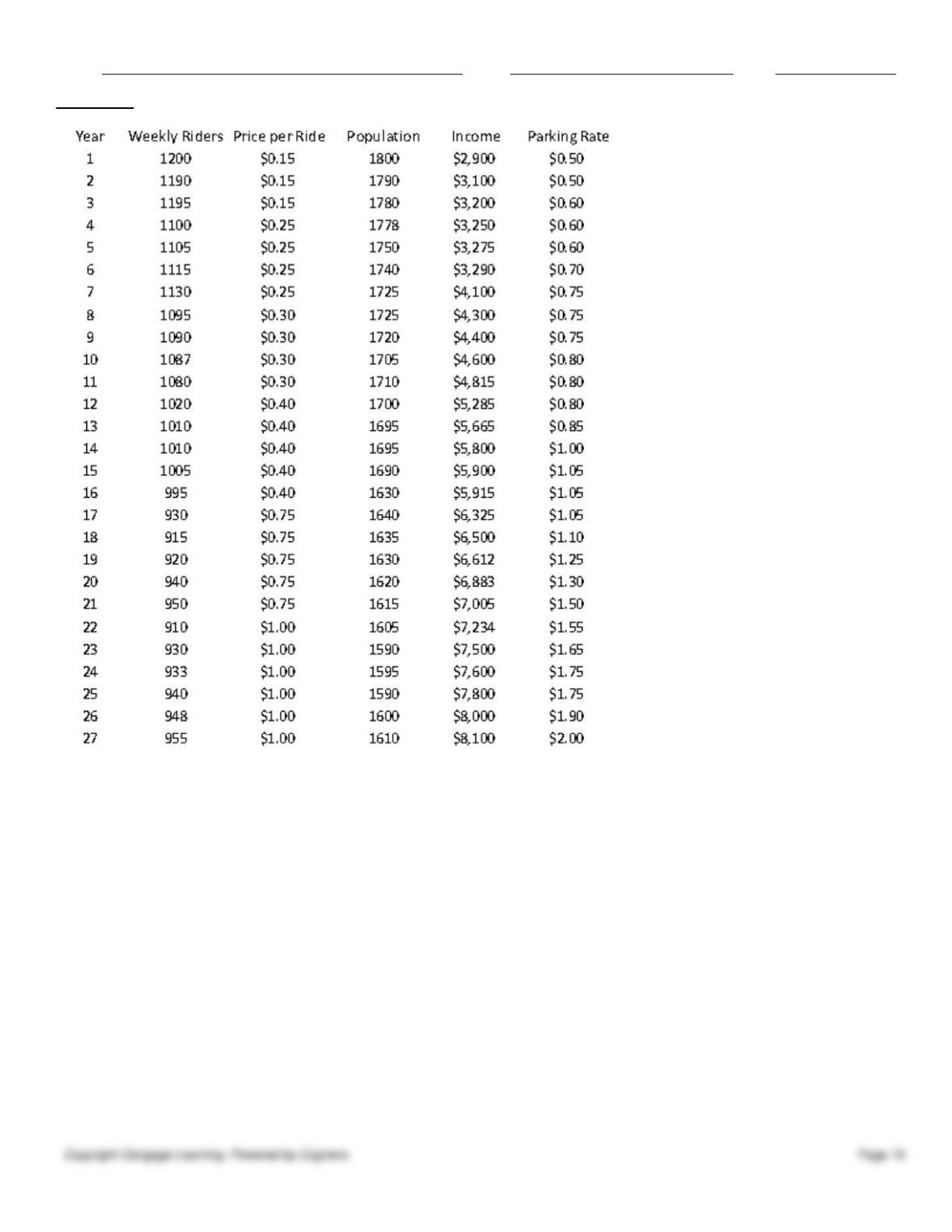
The manager of a commuter rail transportation system was recently asked by his governing board to predict the demand
for rides in the large city served by the transportation network. The system manager has collected data on variables
thought to be related to the number of weekly riders on the city’s rail system. The table shown below contains these data.
Name:
Class:
Date:
chapter 11
The variables “weekly riders” and “population” are measured in thousands, and the variables “price per ride”, “income”,
and “parking rate” are measured in dollars.
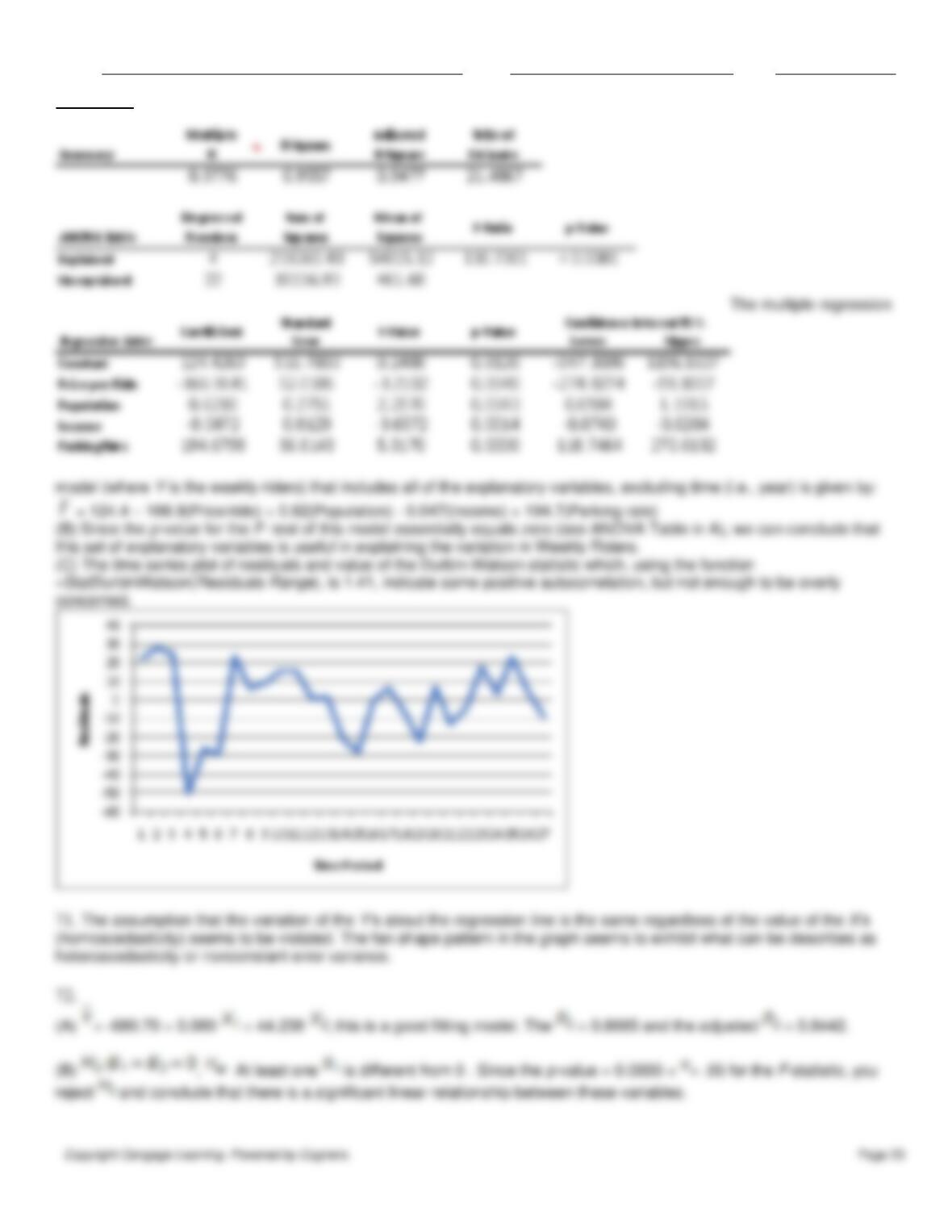
70. (A) Estimate a multiple regression model using all of the available explanatory variables.
(B) Conduct and interpret the result of an F– test on the given model. Employ a 5% level of significance in conducting this
statistical hypothesis test.
(C) Is there evidence of autocorrelated residuals in this model? Explain why or why not.
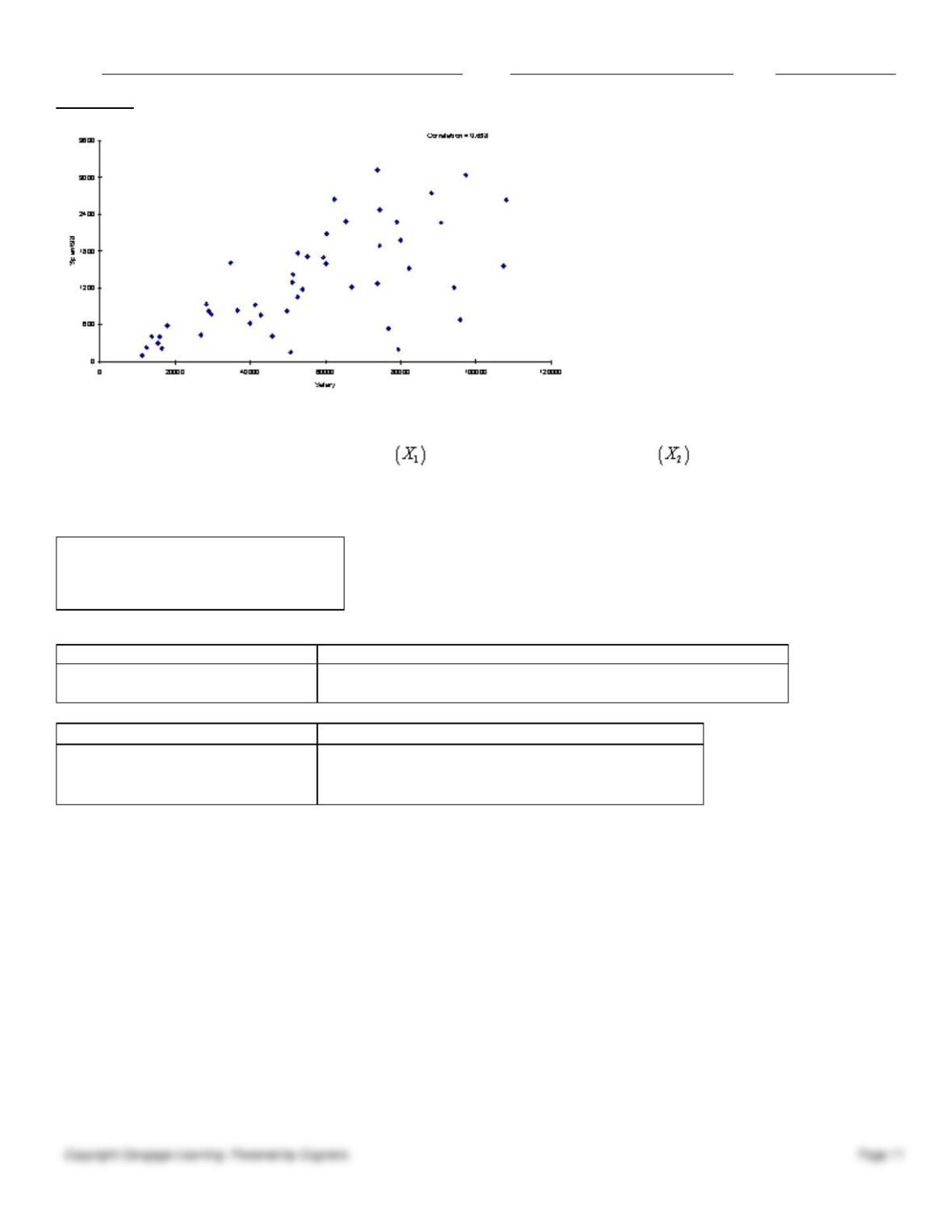
71. Below you will find a scatterplot of data gathered by a mail-order company. The company has been able to obtain the
annual salaries of their customers and the amount that each of these customers spent with the company in 1998. Based
on the scatterplot below, would you conclude that these data meet all four assumptions of regression? Explain your
answer.
Name:
Class:
Date:
chapter 11
A local truck rental company wants to use regression to predict the yearly maintenance expense (Y), in dollars, for a truck
using the number of miles driven during the year and the age of the truck in years at the beginning of the year.
To examine the relationship, the company has gathered the data on 15 trucks and regression analysis has been
conducted. The regression output is presented below.
Summary measures
Multiple R
0.9308
R-Square
0.8665
Adj R-Square
0.8442
StErr of Estimate
87.397
ANOVA Table
Source
df
SS
MS
F
p-value
Explained
2
594690
297345
38.9287
0.0000
Unexplained
12
91658
7638
Regression coefficients
Coefficient
Std Err
t-value
p-value
Constant
-680.70
161.27
-4.2210
0.0012
Miles Driven
0.080
0.015
5.1831
0.0002
Age of Truck
44.238
10.444
4.2359
0.0012
72. (A) Estimate the regression model. How well does this model fit the given data?
(B) Is there a linear relationship between the two explanatory variables and the dependent variable at the 5% significance
level? Explain how you arrived at your answer.
(C) Use the estimated regression model to predict the annual maintenance expense of a truck that is driven 14,000 miles
per year and is 5 years old.
(D) Find a 95% prediction interval for the maintenance expense determined in (C). Use a t-multiple = 2.
(E) Find a 95% confidence interval for the maintenance expense for all trucks sharing the characteristics provided in (C).
Use a t-multiple = 2.
(F) How do you explain the differences between the widths of the intervals in (D) and (E)?
A new online auction site specializes in selling automotive parts for classic cars. The founder of the company believes that
the price received for a particular item increases with its age (i.e., the age of the car on which the item can be used in
years) and with the number of bidders. The Excel multiple regression output is shown below.
Name:
Class:
Date:
chapter 11
Summary measures
Multiple R
0.8391
R-Square
0.7041
Adj R-Square
0.6783
StErr of Estimate
148.828
ANOVA Table
Source
df
SS
MS
F
p-value
Explained
2
1212039.4
606019.7
27.3601
0.0000
Unexplained
23
509444.9
22149.8
Regression coefficients
Coefficient
Std Err
t-value
p-value
Constant
-1242.99
331.204
-3.7529
0.0010
Age of Item
75.017
10.65
7.0459
0.0000
Number of Bidders
13.973
10.44
1.3380
0.1940
73. (A) Estimate a multiple regression model for the data.
(B) Which of the variables in this model have regression coefficients that are statistically different from 0 at the 5%
significance level?
(C) Given your findings in (B), which variables, if any, would you choose to remove from the model estimated in (A)?
Explain your decision.
The information below represents the relationship between the selling price (Y, in $1,000) of a home, the square footage
of the home ( ), and the number of rooms in the home ( ). The data represents 60 homes sold in a particular area of
East Lansing, Michigan and was analyzed using multiple linear regression and simple regression for each independent
variable. The first two tables relate to the multiple regression analysis.
Summary measures
Multiple R
0.9408
R-Square
0.8851
Adj R-Square
0.8660
StErr of Estimate
20.8430
Regression coefficients
Coefficient
Std Err
t-value
p-value
Constant
-13.9705
49.1585
-0.2842
0.7811
Size
7.4336
1.0092
7.3657
0.0000
Number of Rooms
5.3055
8.2767
0.6410
0.5336
The following table is for a simple regression model using only size. ( = 0.8812)
Coefficient
Std Err
t-value
p-value
Constant
14.771
19.691
0.7502
0.4665
Size
7.816
0.796
9.8190
0.0000
The following table is for a simple regression model using only number of rooms. ( = 0.3657)
Coefficient
Std Err
t-value
p-value
Constant
-93.460
108.269
-0.8632
0.4037
Number of Rooms
41.292
15.082
2.7379
0.0169
74. (A) Use the information related to the multiple regression model to determine whether each of the regression
coefficients are statistically different from 0 at a 5% significance level. Summarize your findings.
(B) Test at the 5% significance level the relationship between Y and X in each of the simple linear regression models.
Name:
Class:
Date:
chapter 11
How does this compare to your answer in (A)? Explain.
(C) Is there evidence of multicollinearity in this situation? Explain why or why not.
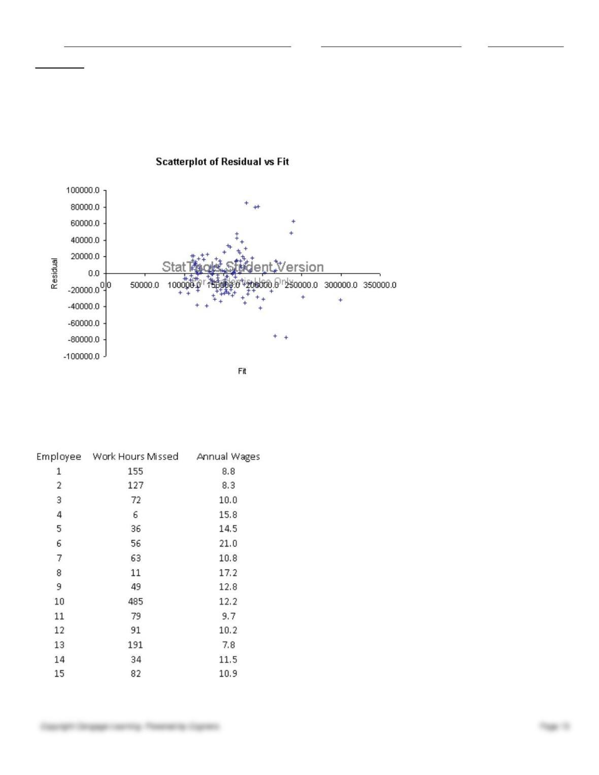
75. Do you see any problems evident in the plot below of residuals versus fitted values from a multiple regression
analysis? Explain your answer.
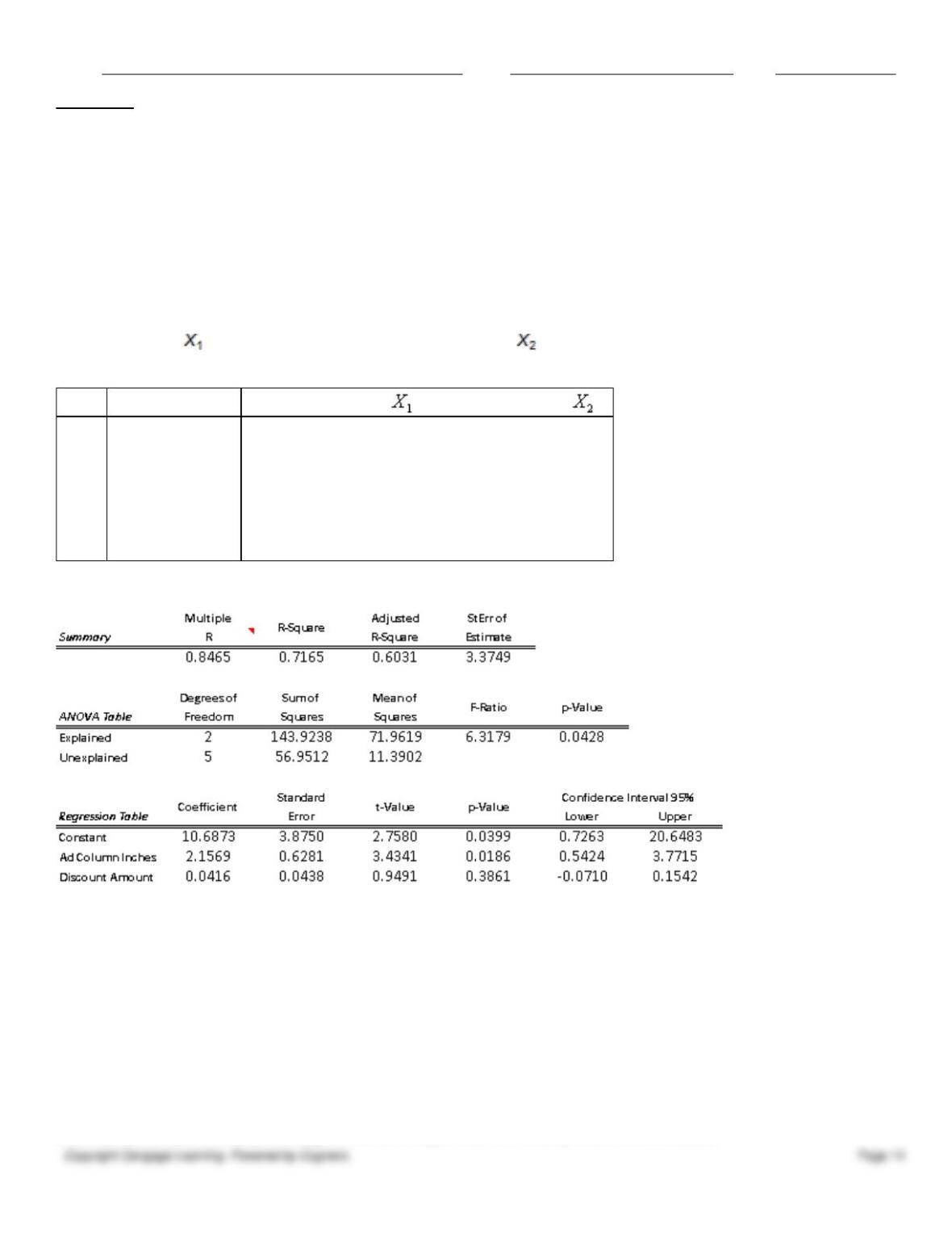
A manufacturing firm wants to determine whether a relationship exists between the number of work-hours an
employee misses per year (Y) and the employee’s annual wages (X), to test the hypothesis that increased
compensation induces better work attendance. The data provided in the table below are based on a random
sample of 15 employees from this organization.
76. (A) Estimate a simple linear regression model using the sample data. How well does the estimated model fit the
sample data?
Name:
Class:
Date:
chapter 11
(B) Perform an F-test for the existence of a linear relationship between Y and X. Use a 5% level of significance.
(C) Plot the fitted values versus residuals associated with the model. What does the plot indicate?
(D) How do you explain the results you have found in (A) through (C)?
(E) Suppose you learn that the 10th employee in the sample has been fired for missing an excessive number of work-
hours during the past year. In light of this information, how would you proceed to estimate the relationship between the
number of work-hours an employee misses per year and the employee’s annual wages, using the available information? If
you decide to revise your estimate of this regression equation, repeat (A) and (B)
The owner of a large chain of health spas has selected eight of her smaller clubs for a test in which she varies the size of
the newspaper ad , and the amount of the initiation fee discount to see how this might affect the number of
prospective members who visit each club during the following week. The results are shown in the table below:
Club
New Visitors (Y)
Ad Column Inches ( )
Discount Amount ( )
1
23
4
$100
2
30
7
20
3
20
3
40
4
26
6
25
5
20
2
50
6
18
5
30
7
17
4
25
8
31
8
80
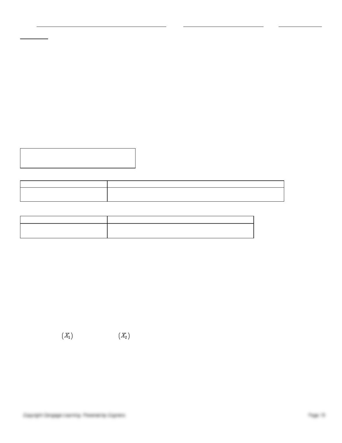
The results of a multiple regression analysis are below.
77. (A) Determine the least-squares multiple regression equation.
(B) Interpret the Y– intercept of the regression equation.
(C) Interpret the partial regression coefficients.
(D) What is the estimated number of new visitors to a club if the size of the ad is 6 column-inches and a $100 discount is
offered?
(E) Determine the approximate 95% prediction interval for the number of new visitors to a given club when the ad is 5
column-inches and the discount is $80.
(F) What is the value for the percentage of variation explained, and exactly what does it indicate?
Name:
Class:
Date:
chapter 11
(G) At the 0.05 level, is the overall regression equation in (A) significant?
(H) Use the 0.05 level in concluding whether each partial regression coefficient differs significantly from zero.
(I Interpret the results of the preceding tests in (H) and (I) in the context of the two explanatory variables described in the
problem.
(J) Construct a 95% confidence interval for each partial regression coefficient in the population regression equation.
A carpet company, which sells and installs carpet, believes that there should be a relationship between the number of
carpet installations that they will have to perform in a given month and the number of building permits that have been
issued within the county where they are located. Below you will find a regression model that compares the relationship
between the number of monthly carpet installations (Y) and the number of building permits that have been issued in a
given month (X). The data represents monthly values for the past 10 months.
Summary measures
Multiple R
0.5682
R-Square
0.3229
StErr of Estimate
9603.23
ANOVA table
Source
df
SS
MS
F
p-value
Explained
1
351824479
351824479
3.8150
0.0866
Unexplained
8
737775521
92221940
Regression coefficients
Coefficient
Std Err
t-value
p-value
Constant
-115076.69
82933.46
-1.3876
0.2027
Permits
53.469
27.375
1.9532
0.0866
78. (A) Estimate the regression model. How well does this model fit the given data?
(B) Yes, there is a linear relationship between the number of carpet installations and the number of building permits
issued at a = 0.10; The p-value = 0.0866 for the F-statistic. You can conclude that there is a significant linear relationship
between these two variables.
(C) The Durbin-Watson statistic for this data was 1.2183. Given this information what would you conclude about the data?
(D) Given your answer in (C), would you recommend modifying the original regression model? If so, how would you
modify it?
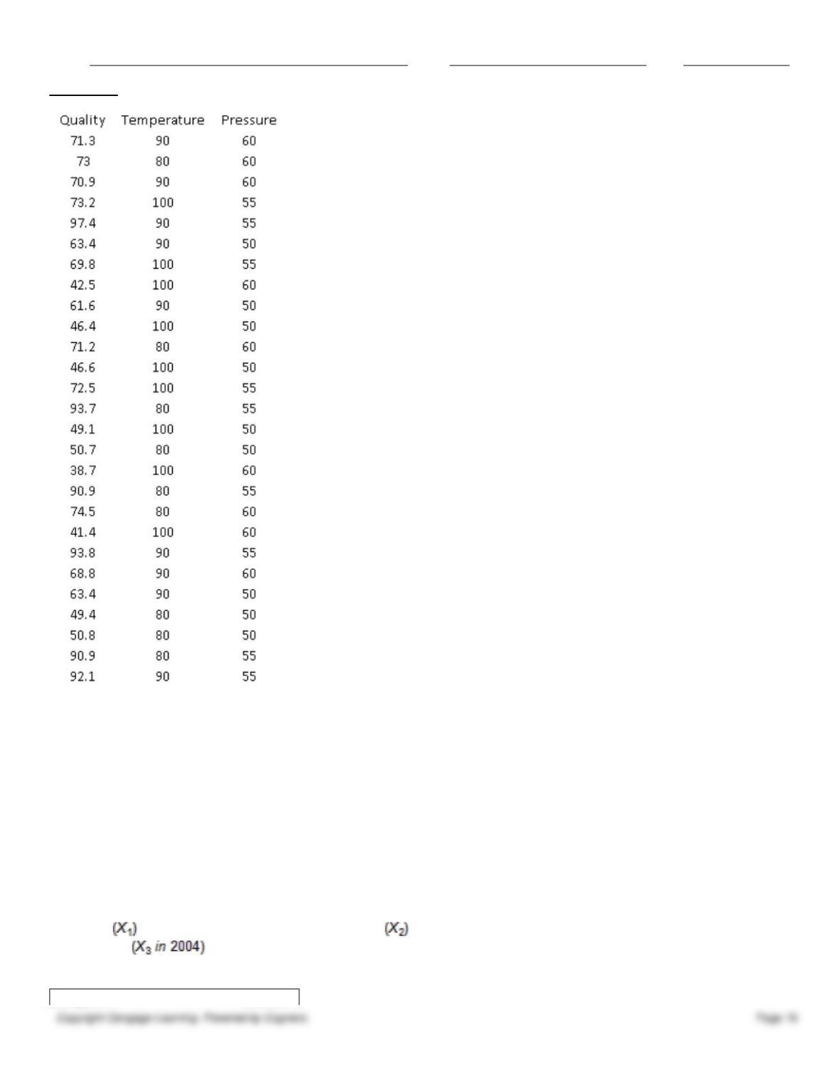
Many companies manufacture products that are at least partially produced using chemicals (for example, paint). In many
cases, the quality of the finished product is a function of the temperature and pressure at which the chemical reactions
take place. Suppose that a particular manufacturer in Texas wants to model the quality (Y) of a product as a function of
the temperature and the pressure at which it is produced. The table below contains data obtained from a
designed experiment involving these variables. Note that the assigned quality score can range from a minimum of 0 to a
maximum of 100 for each manufactured product.
Name:
Class:
Date:
chapter 11
79. (A) Estimate a multiple regression model that includes the two given explanatory variables. Assess this set of
explanatory variables with an F–test, and report a p-value.
(B) Identify and interpret the percentage of variance explained for the model in (A).
(C) Identify and interpret the percentage of variance explained for the model in (B).
(D) Which regression equation is the most appropriate one for modeling the quality of the given product? Bear in mind that
a good statistical model is usually parsimonious.
An internet-based retail company that specializes in audio and visual equipment is interested in creating a model to
determine the amount of money, in dollars, its customers will spend purchasing products from them in the coming year. In
order to create a reliable model, this company has tracked a number of variables on its customers. Below you will find the
Excel output related to several of these variables. This company has tried using the customer’s annual salary for entire
household , the number of children in the household , and if the customer purchased merchandise from them in the
previous year .
Summary measures
Multiple R
0.7825
Name:
Class:
Date:
chapter 11
R-Square
0.6122
Adj R-Square
0.5852
StErr of Estimate
541.70
ANOVA Table
Source
df
SS
MS
F
p-value
Explained
3
19921803
6640601
22.6303
0.0000
Unexplained
43
12617877
293439
Regression coefficients
Coefficient
Std Err
t-value
p-value
Constant
291.243
193.840
1.5025
0.1403
Salary
0.026
0.003
8.0182
0.0000
Number of children
-331.972
79.725
-4.1640
0.0001
Purchase in 2004
281.80
133.82
2.1058
0.0411
80. (A) Estimate the regression model. How well does this model fit the data?
(B) Is there a linear relationship between the explanatory variables and the dependent variable? Explain how you arrived
at your answer at the 5% significance level.
(C) Use the estimated regression model to predict the amount of money a customer will spend if their annual salary is
$45,000, they have 1 child and they were a customer that purchased merchandise in the previous year (2004).
(D) Find a 95% prediction interval for the point prediction calculated in (C). Use a t-multiple = 2.02.
(E) Find a 95% confidence interval for the amount of money spent by all customers sharing the characteristics
described in (C). Use a t-multiple = 2.02.
(F) How do you explain the differences between the widths of the intervals in (D) and (E)?
The owner of a pizza restaurant chain would like to predict the sales of her specialty, the deep-dish Mexican pizza. She
has gathered data on monthly sales of the deep-dish Mexican pizza at her restaurants. She has also gathered information
related to the average price of the deep-dish pizzas, the monthly advertising expenditures and the disposable income per
household in the areas surrounding the restaurants. Below you will find output from the stepwise regression analysis. The
p-value method was used with a cutoff of 0.05.
Summary measures
Multiple R
0.9513
R-Square
0.9049
Adj R-Square
0.8990
StErr of Estimate
3924.53
Regression coefficients
Coefficient
Std Err
t-value
p-value
Constant
-45233.64
8914.72
-5.0740
0.0001
Monthly Adv. Expenditures
1.972
0.160
12.3405
0.0000
81. (A) Summarize the findings of the stepwise regression method using this cutoff value.
(B) When the cutoff value was increased to 0.10, the output below was the result. The table at top left represents the
change when the disposable income variable is added to the model and the table at top right represents the average price
variable being added. The regression model with both added variables is shown in the bottom table. Summarize the
results for this model.
Disposable income variable being added
Name:
Class:
Date:
chapter 11
Summary measures
% Change
Multiple R
0.9608
1.0%
R-Square
0.9232
2.0%
Adj R-Square
0.9130
1.6%
StErr of Estimate
3643.11
–7.2%
Average price variable being added
Summary measures
% Change
Multiple R
0.9723
1.2%
R-Square
0.9454
2.4%
Adj R-Square
0.9337
2.3%
StErr of Estimate
3179.03
–12.7%
Regression coefficients
Coefficient
Std Err
t-value
p-value
Constant
-73971.53
23803.23
-3.1076
0.0077
Monthly Adv. Expenditures
0.952
0.375
2.5387
0.0236
Disposable Income
2.606
0.977
2.6659
0.0184
Average Price
-2056.27
861.342
-2.3873
0.0316
(C) Which model would you recommend using? Why?
A company that makes baseball caps would like to predict the sales of it main product, standard little league caps. The
company has gathered data on monthly sales of caps at all of its retail stores, along with information related to the
average retail price, which varies by location. Below you will find regression output comparing these two variables.
Summary measures
Multiple R
0.5892
R-Square
0.3472
StErr of Estimate
10283.97
ANOVA table
Source
df
SS
MS
F
p-value
Explained
1
899825600
899825600
8.5082
0.0101
Unexplained
16
1692159250
105759953
Regression coefficients
Coefficient
Std Err
t-value
p-value
Constant
147984.44
28831.21
5.1328
0.0001
Average Price
-7370.94
2527.00
-2.9169
0.0101
82. (A) Estimate the regression model. How well does this model fit the given data?
(B) Is there a linear relationship between X and Y at the 5% significance level? Explain how you arrived at your answer.

Name:
Class:
Date:
chapter 11
(C) Use the estimated regression model to predict the number of caps that will be sold during the next month if the
average selling price is $10.
(D) Find a 95% prediction interval for the number of caps determined in (C). Use t- multiple = 2.
(E) Find a 95% confidence interval for the average number of caps sold given an average selling price of $10. Use a t–
multiple = 2.
(F) How do you explain the differences between the widths of the intervals in (D) and (E)?
Name:
Class:
Date:
chapter 11
Answer Key
Name:
Class:
Date:
chapter 11
Name:
Class:
Date:
chapter 11
Name:
Class:
Date:
chapter 11
heteroscedasticity or nonconstant error variance.
Name:
Class:
Date:
chapter 11
residuals, so there is no major problem evident.
Name:
Class:
Date:
chapter 11
Name:
Class:
Date:
chapter 11
Name:
Class:
Date:
chapter 11
Name:
Class:
Date:
chapter 11
(C) It seems that there is some increased benefit by using the second (expanded) model. In going from the first to the
Name:
Class:
Date:
chapter 11