Page 1
1.
The changes in the economy of Ft. Myers, Florida, between 2003 and 2010 provide an
example of:
A)
the risk associated with an agricultural economy.
B)
positive and negative multiplier effects.
C)
how public assistance programs can stimulate the economy.
D)
the benefits of government budget surpluses.
2.
The real estate market in Ft. Myers, Florida, had collapsed by 2008 because:
A)
houses were overpriced.
B)
most Floridians prefer to rent apartments rather than buy houses.
C)
hurricanes damaged so much property.
D)
climate change has made much of the retiree population leave Florida.
3.
The main reason that speculators bought houses in Ft. Myers in the early 2000s was:
A)
to profit by reselling them at much higher prices.
B)
to live in them.
C)
to demolish them and build a shopping mall.
D)
to rent them to students.
4.
The expansion and collapse of the housing market in Ft. Myers between 2003 and 2010
is primarily an example of how:
A)
too much government regulation is harmful to the economy.
B)
changes in investment spending can affect consumer spending and the entire
economy.
C)
immigration affects local economies.
D)
high tax rates can decrease economic activity in an area.
5.
The marginal propensity to consume is:
A)
increasing if the marginal propensity to save is increasing.
B)
the proportion of total disposable income that the average family consumes.
C)
the change in consumer spending divided by the change in aggregate disposable
income.
D)
the change in consumer spending minus the change in aggregate disposable
income.
Page 2
6.
The marginal propensity to consume equals the:
A)
proportion of consumer spending as a function of aggregate disposable income.
B)
change in savings divided by the change in aggregate disposable income.
C)
ratio of the change in consumer spending to the change in aggregate disposable
income.
D)
change in savings divided by the change in consumer spending.
7.
The marginal propensity to save plus the marginal propensity to consume must equal:
A)
zero.
B)
one.
C)
income.
D)
savings.
8.
If the MPS = 0.1, then the multiplier equals:
A)
1.
B)
5.
C)
9.
D)
10.
9.
If the multiplier equals 4, then the marginal propensity to save must be equal to:
A)
0.25.
B)
0.5.
C)
0.75.
D)
the marginal propensity to consume.
10.
Suppose that the marginal propensity to consume is 0.8 and investment spending
increases by $100 billion. The increase in real GDP is:
A)
$100 billion, the same amount as investment spending.
B)
$125 billion, composed of $100 billion in investment spending and $25 billion in
consumption.
C)
$80 billion, composed of $100 billion in investment spending and a decrease in
consumption of $20 billion.
D)
$500 billion, composed of $100 billion in investment spending and $400 billion in
consumption.
11.
If the marginal propensity to save is 0.3, the size of the multiplier is:
A)
3.3.
B)
2.3.
C)
1.3.
D)
0.7.
Page 3
12.
The marginal propensity to save is:
A)
savings divided by aggregate income.
B)
the fraction of an additional dollar of disposable income that is saved.
C)
1 + MPC.
D)
savings divided by aggregate income, or 1 + MPC.
13.
The multiplier is:
A)
1 / (1 – MPC).
B)
MPS / MPC.
C)
1 / (MPC).
D)
1(1 + MPC).
14.
If the marginal propensity to consume is 0.8, then the multiplier is:
A)
4.
B)
5.
C)
8.
D)
10.
15.
The marginal propensity to consume (MPC) equals the change in _____ divided by the
change in _____.
A)
consumer spending; disposable income
B)
consumer spending; investment spending
C)
consumer spending; gross domestic product
D)
disposable income; consumer spending
16.
If disposable income increases by $5 billion and consumer spending increases by $4
billion, the marginal propensity to consume equals:
A)
20.
B)
0.8.
C)
1.25.
D)
9.
17.
Suppose the marginal propensity to consume equals 0.9 and investment spending
increases by $50 billion. Assuming no taxes and no trade, real GDP will _____ by
_____.
A)
increase; $450 billion
B)
increase; $90 billion
C)
increase; $500 billion
D)
decrease; $500 billion
Page 4
18.
Assuming no taxes and no trade, the multiplier equals:
A)
MPC / MPS.
B)
1 / (1 – MPS).
C)
MPC + MPS.
D)
1 / (1 – MPC).
19.
Suppose that a financial crisis decreases investment spending by $100 billion and the
marginal propensity to consume is 0.8. Assuming no taxes and no trade, real GDP will
_____ by _____.
A)
decrease; $500 billion
B)
decrease; $200 billion
C)
decrease; $800 billion
D)
increase; $400 billion
20.
The marginal propensity to consume is the change in _____ divided by the change in
_____.
A)
savings; disposable income
B)
disposable income; consumption
C)
disposable income; savings
D)
consumption; disposable income
21.
If your disposable income increases from $10,000 to $15,000 and your consumption
increases from $9,000 to $12,000, your marginal propensity to consume is:
A)
0.2.
B)
0.4.
C)
0.6.
D)
0.8.
22.
If your disposable personal income increases from $10,000 to $15,000 and your
consumption increases from $9,000 to $13,000, your marginal propensity to consume is:
A)
0.2.
B)
0.4.
C)
0.6.
D)
0.8.

Page 5
23.
The marginal propensity to consume plus the marginal propensity to save must:
A)
equal each other.
B)
equal 1.
C)
be less than 1.
D)
be greater than 1.
24.
The value of the marginal propensity to consume is:
A)
1.
B)
greater than 1.
C)
between 0 and 1.
D)
less than 0 and greater than –1.
25.
An increase in the marginal propensity to consume:
A)
increases the multiplier.
B)
shifts the autonomous investment line upward.
C)
decreases the multiplier.
D)
shifts the autonomous investment line downward.
26.
Which of the following most accurately depicts the formula for the expenditure
multiplier?
A)
and
11
MPC MPS
MPS MPC−−
B)
11
and 1MPC MPS−
C)
11
and 1MPS MPC−
D)
and
MPS MPC
MPC MPS
27.
If MPC = 0.9, the multiplier is:
A)
10.
B)
90.
C)
9.
D)
1.
Page 6
28.
The _____ the _____, the _____ the multiplier.
A)
smaller; level of wealth; bigger
B)
bigger; marginal propensity to save; bigger
C)
bigger; marginal propensity to consume; smaller
D)
bigger; marginal propensity to consume; bigger
29.
Suppose investment spending increases by $50 billion and as a result the equilibrium
income increases by $200 billion. The investment multiplier is:
A)
8.
B)
10.
C)
4.
D)
0.25.
30.
Suppose investment spending increases by $50 billion and as a result the equilibrium
income increases by $200 billion. The value of the marginal propensity to consume is:
A)
0.8.
B)
0.4.
C)
0.75.
D)
4.
31.
If the multiplier is 4 and investment spending falls by $100 billion, the change in real
GDP will be:
A)
–$400 billion.
B)
$400 billion.
C)
$25 billion.
D)
–$25 billion.
32.
Suppose the government increases spending by $100 billion as a stimulus package. If
the marginal propensity to consume is 0.6, then real GDP will:
A)
decrease by $250 billion.
B)
increase by $250 billion.
C)
increase by $600 billion.
D)
decrease by $400 billion.
Page 7
33.
Suppose that the U.S. economy is in a severe recession. Most households are trying to
save more of their income than before. This increase in private savings will lead to:
A)
an increase in real GDP, as more savings means more funds for business
investment.
B)
a fall in real GDP, as more savings means people will spend less.
C)
no change in real GDP, because there is no savings multiplier.
D)
an increase in real GDP, as an increase in savings will make people wealthier.
34.
If the marginal propensity to save is small, it will:
A)
make the multiplier smaller.
B)
make the multiplier larger.
C)
not affect the value of the multiplier.
D)
increase the interest rate.
35.
The marginal propensity to consume is the increase in consumer spending when _____
increase(s) by $1.
A)
investment spending
B)
taxes
C)
disposable income
D)
savings
36.
The marginal propensity to save is the increase in household savings when _____
increase(s) by $1.
A)
investment spending
B)
taxes
C)
consumption
D)
disposable income
37.
In a simple economy with no taxes, government spending, exports, or imports, if
disposable income increases by $100 and $70 is consumed, _____ is saved.
A)
$30
B)
$70
C)
$100
D)
$170
Page 8
38.
In a simple economy with no taxes, government spending, exports, or imports, if
disposable income increases by $100 and $30 is saved, _____ is consumed.
A)
$30
B)
$70
C)
$100
D)
$170
39.
A $50 million increase in investment spending will eventually cause equilibrium real
GDP to:
A)
decrease by $50 million.
B)
increase by $50 million.
C)
increase by more than $50 million.
D)
increase by less than $50 million.
40.
A $70 million decrease in investment spending will cause real GDP to:
A)
decrease by $70 million.
B)
increase by $70 million.
C)
decrease by less than $70 million.
D)
decrease by more than $70 million.
41.
An initial change in the desired level of spending by firms, households, or government
at a given level of real GDP is a(n):
A)
autonomous change in aggregate spending.
B)
multiplier-induced change in spending.
C)
endogenous spending.
D)
budget surplus.
42.
In an economy with no taxes or imports, if the marginal propensity to save is 0.2, the
marginal propensity to consume must be:
A)
0.2
B)
0.8
C)
1.2
D)
0.16
43.
In an economy with no taxes or imports, if the marginal propensity to consume is 0.7,
the marginal propensity to save must be:
A)
1.7
B)
0.7
C)
0.3
D)
0.21
Page 9
44.
In an economy with no taxes or imports, if the marginal propensity to consume
increases, the marginal propensity to save will:
A)
increase.
B)
decrease.
C)
remain constant.
D)
fluctuate randomly.
45.
In an economy with no taxes or imports, if the marginal propensity to save decreases,
the marginal propensity to consume will:
A)
increase.
B)
decrease.
C)
remain constant.
D)
fluctuate randomly.
46.
In an economy with no taxes or imports, if disposable income increases by $1,000 and
consumption increases by $600, the marginal propensity to consume is:
A)
$600.
B)
$400.
C)
1.67.
D)
0.60.
47.
In an economy with no taxes or imports, if disposable income increases by $1,000 and
consumption increases by $600, the marginal propensity to save is:
A)
$600.
B)
$400.
C)
2.5.
D)
0.40.
48.
In an economy with no taxes or imports, if disposable income increases by $1,000 and
consumption increases by $600, the multiplier is:
A)
$600.
B)
0.6.
C)
2.5.
D)
0.40.
Page 10
49.
In an economy with no taxes and no imports, disposable income increases from $2,000
to $3,000. If consumption increases from $1,500 to $2,100, the marginal propensity to
consume is:
A)
$600.
B)
0.71.
C)
0.60.
D)
0.50.
50.
In an economy with no taxes and no imports, disposable income increases from $2,000
to $3,000. If consumption increases from $1,500 to $2,100, the marginal propensity to
save is:
A)
$600.
B)
$400.
C)
0.80.
D)
0.40.
51.
In an economy with no taxes and no imports, disposable income increases from $2,000
to $3,000. If consumption increases from $1,500 to $2,100, the multiplier is:
A)
6.
B)
2.5.
C)
0.60.
D)
0.40.
52.
In an economy with no taxes and no imports, disposable income decreases from $6,000
to $4,000. If consumption decreases from $4,500 to $3,000, the marginal propensity to
consume is:
A)
–0.75.
B)
–0.20.
C)
0.75.
D)
1.
53.
In an economy with no taxes and no imports, disposable income decreases from $6,000
to $4,000. If consumption decreases from $4,500 to $3,000, the marginal propensity to
save is:
A)
0.25.
B)
–0.25.
C)
1.125.
D)
0.75.
Page 11
54.
In an economy with no taxes and no imports, disposable income decreases from $6,000
to $4,000. If consumption decreases from $4,500 to $3,000, the multiplier is:
A)
0.25.
B)
4.
C)
1.125.
D)
–4.
55.
If the marginal propensity to consume increases, the multiplier will:
A)
increase.
B)
decrease.
C)
remain constant.
D)
fluctuate randomly.
56.
If the marginal propensity to save increases, the multiplier will:
A)
increase.
B)
decrease.
C)
remain constant.
D)
fluctuate randomly.
57.
If the marginal propensity to consume is 0.8, the multiplier is:
A)
0.8.
B)
0.2.
C)
1.25.
D)
5.
58.
If the marginal propensity to consume is 0.5, the multiplier is:
A)
5.
B)
2.
C)
1.
D)
0.5.
59.
If the marginal propensity to save is 0.2, the multiplier is:
A)
0.8.
B)
0.2.
C)
1.25.
D)
5.
Page 12
60.
If the marginal propensity to save is 0.5, the multiplier is:
A)
5.
B)
2.
C)
1.
D)
0.5.
61.
If the multiplier is 4, the marginal propensity to consume is:
A)
3.
B)
0.80.
C)
0.75.
D)
0.25.
62.
If the multiplier is 4, the marginal propensity to save is:
A)
3.
B)
0.80.
C)
0.75.
D)
0.25.
63.
If the multiplier is 4 and autonomous government spending increases by $100 billion,
real GDP will:
A)
increase by $400 billion.
B)
decrease by $400 billion.
C)
increase by $100 billion.
D)
increase by $25 billion.
64.
If the multiplier is 4 and autonomous government spending decreases by $100 billion,
real GDP will:
A)
increase by $400 billion.
B)
decrease by $400 billion.
C)
increase by $100 billion.
D)
increase by $25 billion.
Page 13
Use the following to answer questions 65-69:
Figure: Consumption and Real GDP
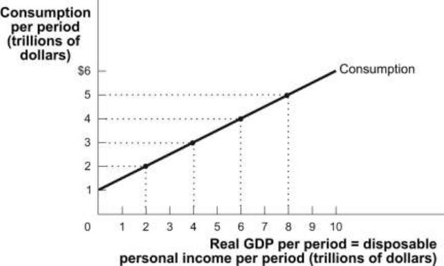
65.
(Figure: Consumption and Real GDP) Look at the figure Consumption and Real GDP.
The slope of the consumption function is called the:
A)
marginal propensity to save.
B)
average propensity to consume.
C)
marginal propensity to consume.
D)
marginal consumption increment.
66.
(Figure: Consumption and Real GDP) Look at the figure Consumption and Real GDP.
The marginal propensity to consume is:
A)
0.
B)
0.5.
C)
1.0.
D)
2.0.
67.
(Figure: Consumption and Real GDP) Look at the figure Consumption and Real GDP. If
real GDP is $4 trillion, consumption is _____ trillion.
A)
$0.75
B)
$1
C)
$3
D)
$4
Page 14
68.
(Figure: Consumption and Real GDP) Look at the figure Consumption and Real GDP. If
real GDP is $12 trillion, consumption is _____ trillion.
A)
$5
B)
$7
C)
$9
D)
$11
69.
(Figure: Consumption and Real GDP) Look at the figure Consumption and Real GDP. If
real GDP is $8 trillion, consumption is _____ trillion and savings is _____ trillion.
A)
$4; $4
B)
$5; $3
C)
$6; $2
D)
$7; $1
70.
You and a coworker have been trying to develop a linear equation that describes the
local household consumption function. Your coworker has sent you a very short email
that simply says he has finished the project and the consumption function is C = 100 +
0.75(YD). Your job is to explain this result to your supervisor. According to this
consumption function, what is the marginal propensity to consume?
A)
100
B)
0.75
C)
4
D)
0.25
71.
You and a coworker have been trying to develop a linear equation that describes the
local household consumption function. Your coworker has sent you a very short email
that simply says he has finished the project and the consumption function is C = 100 +
0.75(YD). Your job is to explain this result to your supervisor. According to this
consumption function, how much consumption spending would occur if a household
had disposable income of $1,000?
A)
$750
B)
$4,000
C)
$850
D)
$350
72.
Suppose the marginal propensity to consume changes from 0.75 to 0.9. How will this
affect the consumption function?
A)
The slope will get steeper.
B)
Autonomous consumption will increase.
C)
The function will shift downward.
D)
The slope will get steeper and autonomous consumption will increase.
Page 15
Use the following to answer questions 73-78:
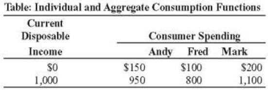
73.
(Table: Individual and Aggregate Consumption Functions) Look at the table Individual
and Aggregate Consumption Functions. Which of the following represents Andy’s
individual consumption function?
A)
C = 0.15YD
B)
C = 150 + 0.5YD
C)
C = 150 + 0.8YD
D)
C = 0.95YD
74.
(Table: Individual and Aggregate Consumption Functions) Look at the table Individual
and Aggregate Consumption Functions. Which of the following represents Fred’s
individual consumption function?
A)
C = 100 + 0.7YD
B)
C = 100 + 0.5YD
C)
C = 150 + 0.8YD
D)
C = 0.80YD
75.
(Table: Individual and Aggregate Consumption Functions) Look at the table Individual
and Aggregate Consumption Functions. Which of the following represents Mark’s
individual consumption function?
A)
C = 200 + 1.1YD
B)
C = 450 + 0.5YD
C)
C = 0.8YD
D)
C = 200 + 0.9YD
76.
(Table: Individual and Aggregate Consumption Functions) Look at the table Individual
and Aggregate Consumption Functions. Autonomous consumption in the aggregate
consumption function is:
A)
$450.
B)
$200.
C)
$150.
D)
$100.
Page 16
77.
(Table: Individual and Aggregate Consumption Functions) The marginal propensity to
consume in the aggregate consumption function is:
A)
0.5.
B)
0.7.
C)
0.8.
D)
0.9.
78.
(Table: Individual and Aggregate Consumption Functions) Which of the following
represents the aggregate consumption function?
A)
C = 450 + 0.7YD
B)
C = 150 + 0.9YD
C)
C = 250 + 0.8YD
D)
C = 450 + 0.8YD
Use the following to answer questions 79-81:
Figure: Consumption and Disposable Personal Income
Page 17
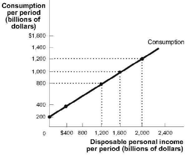
79.
(Figure: Consumption and Disposable Personal Income) Look at the figure
Consumption and Disposable Personal Income. When disposable personal income is
$1,200 billion, consumption is _____ billion.
A)
$600
B)
$800
C)
$1,200
D)
$2,000
80.
(Figure: Consumption and Disposable Personal Income) Look at the figure
Consumption and Disposable Personal Income. When disposable personal income is
$2,000 billion, consumption is _____ billion.
A)
$400
B)
$1,000
C)
$1,200
D)
$1,600
81.
(Figure: Consumption and Disposable Personal Income) Look at the figure
Consumption and Disposable Personal Income. The slope of the consumption function
is:
A)
0.25.
B)
0.50.
C)
0.60.
D)
0.67.
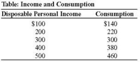
Use the following to answer questions 82-84:
82.
(Table: Income and Consumption) Look at the table Income and Consumption. When
disposable personal income is $200, the marginal propensity to consume is:
A)
0.00.
B)
0.20.
C)
0.80.
D)
1.40.
Page 18
83.
(Table: Income and Consumption) Look at the table Income and Consumption. When
disposable personal income is $300, the marginal propensity to consume is:
A)
0.80.
B)
0.92.
C)
0.95.
D)
1.00.
84.
(Table: Income and Consumption) Look at the table Income and Consumption. When
disposable personal income is $400, the level of personal savings is:
A)
–$40.
B)
–$20.
C)
$0.
D)
$20.
85.
The most important determinant of consumer spending is:
A)
the government budget deficit or surplus.
B)
the price of gasoline.
C)
the trade deficit.
D)
disposable income.
Use the following to answer questions 86-90:
Scenario: Consumption Spending
Suppose that the consumption function is C = $500 + 0.8 × YD, where YD is disposable income.
86.
(Scenario: Consumption Spending) Look at the scenario Consumption Spending.
Autonomous consumption is:
A)
$500.
B)
0.
C)
four-fifths of disposable income.
D)
$1,300 if disposable income is $1,000.
87.
(Scenario: Consumption Spending) Look at the scenario Consumption Spending. The
marginal propensity to consume is:
A)
$500.
B)
0.
C)
0.8.
D)
0.2.
Page 19
88.
(Scenario: Consumption Spending) Look at the scenario Consumption Spending. The
marginal propensity to save is:
A)
$500.
B)
0.
C)
0.8.
D)
0.2.
89.
(Scenario: Consumption Spending) Look at the scenario Consumption Spending. If
income increases by $2,000, consumption will increase by:
A)
$500.
B)
$2,000.
C)
$1,600.
D)
$400.
90.
(Scenario: Consumption Spending) Look at the scenario Consumption Spending. If
disposable income is $1,000, savings is:
A)
–$500.
B)
$1,300.
C)
–$300.
D)
$300.
91.
When David has no income, he spends $500. If his income increases to $2,000, he
spends $1,900. Which of the following represents his consumption function?
A)
C = 1.2 × YD
B)
C = 0.95 × YD
C)
C = $500 + 0.7 × YD
D)
C = $500 + 1,000 × YD
92.
Consumer spending in the United States normally accounts for approximately _____ of
the economy.
A)
one-third
B)
one-half
C)
two-thirds
D)
three-fourths

Page 20
93.
The following is an algebraic representation of the consumption function: C = A + MPC
× YD. Which of the following represents the slope of the function?
A)
C
B)
A
C)
MPC
D)
YD
Use the following to answer question 94:
Table: Individual Consumption for Bob
Disposable Income
Bob
$ 0
$ 9,000
10,000
13,000
94.
(Table: Individual Consumption Function for Bob) Look at the table Individual
Consumption Function for Bob. The marginal propensity to consume and autonomous
consumption are _____ and _____, respectively, for Bob.
A)
0.6; $10,000
B)
0.4; $13,000
C)
0.6; $9,000
D)
0.4; $9,000
95.
The most important factor affecting a household’s consumer spending is:
A)
its expected disposable income.
B)
its current disposable income.
C)
its wealth.
D)
the interest rate.
96.
In the consumption function, an individual household’s consumer spending:
A)
is positively related to its current disposable income.
B)
is negatively related to its autonomous consumption and its marginal propensity to
consume.
C)
is positively related to the interest rate.
D)
is determined by the accelerator principle.
Page 21
97.
If the marginal propensity to consume is 0.5, individual autonomous consumption is
$10,000, and disposable income is $40,000, then individual consumption spending is:
A)
$20,000.
B)
$25,000.
C)
$30,000.
D)
$45,000.
98.
Assuming that A represents autonomous consumption and YD represents disposable
income, for the economy as a whole:
A)
C = MPC + (A × YD).
B)
C = A + (MPC × YD).
C)
C = (A + MPC) × YD.
D)
C = (A – MPS) + (MPC × YD).
99.
The marginal propensity to consume is _____ of the consumption function.
A)
the slope
B)
the intercept
C)
the inverse
D)
independent
100.
If aggregate consumption equals $100 million + 0.75 × YD, then the marginal
propensity to consume is:
A)
0.75.
B)
0.25.
C)
$75 million.
D)
$100 million.
101.
If aggregate consumption equals $100 million + 0.75 × YD, then the marginal
propensity to save is:
A)
0.75.
B)
0.25.
C)
–$75 million.
D)
–$100 million.
102.
If the aggregate consumption equals $100 million + 0.75 × YD, then autonomous
consumption is:
A)
0.75.
B)
0.25.
C)
$75 million.
D)
$100 million.
Page 22
103.
The aggregate consumption function:
A)
relates household consumption to interest rates.
B)
describes what people would like to buy.
C)
describes the relationship of spending to family wealth.
D)
relates disposable income to total consumer spending.
104.
In the equation C = A + MPC × YD, _____ represents autonomous consumption.
A)
C
B)
A
C)
MPC
D)
YD
105.
David receives a tax refund of $800. He spends $600 and saves $200. David’s marginal
propensity to consume is:
A)
0.6.
B)
0.75.
C)
0.25.
D)
0.20.
106.
If the marginal propensity to consume is greater than zero but less than one, when
disposable income rises by $1, consumption will:
A)
not be affected.
B)
rise by more than $1.
C)
rise by less than $1.
D)
rise by exactly $1.
107.
If the consumption function is plotted on the vertical axis of a graph with disposable
income on the horizontal axis:
A)
the slope of the line will be negative and determined by the marginal propensity to
save.
B)
the horizontal axis intercept will be determined by the level of autonomous
consumption.
C)
the slope of the line will be positive and determined by the marginal propensity to
consume.
D)
the vertical axis intercept will be determined by the marginal propensity to save.
Page 23
108.
The marginal propensity to consume equals:
A)
consumption divided by disposable income.
B)
a change in consumption divided by a change in disposable income.
C)
income divided by consumption.
D)
a change in income divided by a change in consumption.
109.
If the marginal propensity to save decreases from 0.6 to 0.5:
A)
the slope of the consumption function increases from 0.4 to 0.5.
B)
the vertical axis intercept of the consumption function changes from 0.6 to 0.5.
C)
the slope of the consumption function decreases from 0.6 to 0.5.
D)
the horizontal axis intercept of the consumption function changes from 0.4 to 0.5.
110.
Consider the simple economy of Behr, whose government does not tax its citizens. The
consumption function of Behr is given by C = 500 + 0.80Y, where Y is income. The
autonomous consumer spending in this economy is:
A)
1,000.
B)
800.
C)
500.
D)
not possible to calculate.
111.
Consider the simple economy of Behr, whose government does not tax its citizens. The
consumption function of Behr is given by C = 500 + 0.80Y, where Y is income. The
marginal propensity to consume in Behr is:
A)
0.75.
B)
500.
C)
0.80.
D)
1.
112.
If disposable income increases:
A)
the consumption function will shift upward.
B)
there will be a rightward movement along the consumption function.
C)
there will be a leftward movement along the consumption function.
D)
the consumption function will shift downward.
113.
If disposable income increases by $1,000 and consumer spending increases by $800,
then the marginal propensity to consume is:
A)
0.8.
B)
1.
C)
1.25.
D)
0.75.

Page 24
114.
If the marginal propensity to consume is 0.75, then the marginal propensity to save is:
A)
1.75.
B)
0.25.
C)
–0.25.
D)
1.25.
Use the following to answer questions 115-116:
Table: Disposable Income and Consumption
Disposable Income
(in Billions)
Consumer Spending
(in Billions)
$ 0
$100
200
220
400
340
600
460
800
580
1,000
700
115.
(Table: Disposable Income and Consumption) Look at the table Disposable Income and
Consumption. Autonomous consumer spending is:
A)
200.
B)
100.
C)
120.
D)
0.
116.
(Table: Disposable Income and Consumption) Look at the table Disposable Income and
Consumption. The marginal propensity to consume equals:
A)
0.8.
B)
2.
C)
1.2.
D)
0.6.
117.
Consider a simple economy: MPC = 0.75, income = $400 billion, and aggregate
consumption spending = $400 billion. Autonomous consumption is:
A)
0.
B)
$100 billion.
C)
$300 billion.
D)
$200 billion.
Page 25
118.
The consumption function will shift up if:
A)
households expect an increase in the minimum wage.
B)
households expect a decrease in the minimum wage.
C)
the marginal propensity to consume decreases.
D)
the marginal propensity to save increases.
119.
If other things are equal, expectations of lower disposable income would _____ and
shift the consumption function _____.
A)
increase autonomous consumption; up
B)
decrease the marginal propensity to consume; down
C)
decrease autonomous consumption; down
D)
increase the marginal propensity to consume; up
120.
The marginal propensity to consume is 0.5, aggregate autonomous consumption is
$10,000, and aggregate disposable income is $40,000. If disposable income is expected
to increase, the aggregate consumption function might take the form of:
A)
C = 10,000 + (40,000 × 0.5).
B)
C = 12,000 + (40,000 × 0.5).
C)
C = 10,000 + (40,000 × 0.7).
D)
C = 10,000 + (42,000 × 0.5).
121.
When future disposable income rises, current consumption:
A)
falls.
B)
rises.
C)
is unaffected.
D)
is autonomous.
122.
Which of the following will shift the aggregate consumption function UPWARD?
A)
Disposable income rises.
B)
Consumer expectations turn more pessimistic.
C)
The stock market is strong and wealth is rising.
D)
Disposable income falls.
Page 26
Use the following to answer questions 123-124:
Figure: Consumption Functions
123.
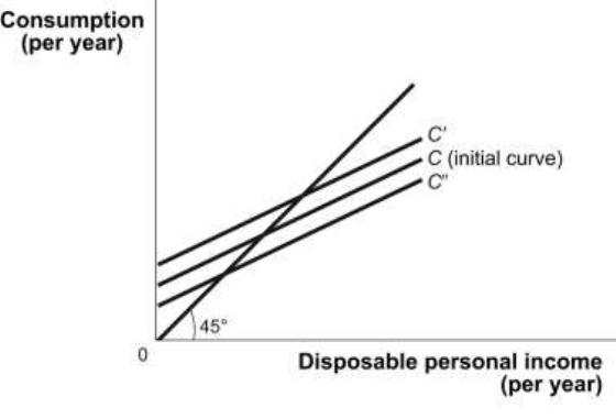
(Figure: Consumption Functions) Look at the figure Consumption Functions. An
economy’s consumption function would shift from curve C to curve C when there is
a(n):
A)
decrease in wealth.
B)
decrease in the price level.
C)
increase in expected disposable income.
D)
increase in wealth.
124.
(Figure: Consumption Functions) Look at the figure Consumption Functions. An
economy’s consumption function would shift from curve C to curve C
when there is
a(n):
A)
increase in expected disposable income.
B)
decrease in expected GDP growth estimates.
C)
drop in wealth.
D)
increase in the unemployment rate.
125.
An increase in the wealth of households, all other things unchanged, will result in _____
the aggregate consumption function.
A)
no effect on
B)
an upward shift in
C)
a downward shift of
D)
a movement to the right along
Page 27
126.
An upward shift in the aggregate consumption function can be caused by:
A)
expectations of higher incomes.
B)
expectations of less income.
C)
a stock market crash.
D)
a reduction in the wealth of households.
127.
A downward shift in the consumption function can be caused by:
A)
expectations of higher incomes.
B)
an increase in the marginal propensity to consume.
C)
a decline in consumer wealth.
D)
an increase in the wealth of households.
128.
An upward shift in the consumption function can be caused by:
A)
an increase in consumer wealth.
B)
a drop in consumer wealth.
C)
pessimistic expectations.
D)
an increase in disposable personal income.
129.
A downward shift in the consumption function can be caused by:
A)
a decrease in disposable income.
B)
an increase in disposable income.
C)
expectations of higher permanent income.
D)
a decrease in wealth.
130.
If the stock market crashes:
A)
the aggregate consumption function will shift up.
B)
the aggregate consumption function will shift down.
C)
unplanned inventory investment will be negative.
D)
GDP will increase.
131.
Which of the following is NOT a determinant of consumer spending?
A)
disposable income
B)
expected disposable income
C)
wealth
D)
investment spending
Page 28
132.
If other things are equal, an increase in aggregate wealth will _____ and shift the
consumption function _____.
A)
increase autonomous consumption; up
B)
decrease the marginal propensity to consume; down
C)
decrease autonomous consumption; down
D)
increase the marginal propensity to consume; up
133.
The aggregate consumption function depends on:
A)
disposable income.
B)
expected disposable income.
C)
wealth.
D)
disposable income, expected disposable income, and wealth.
134.
According to the life-cycle hypothesis, wealth affects consumer spending because:
A)
wealthier people have higher incomes.
B)
wealthier people have better connections to buy in-demand goods.
C)
people try to smooth their consumption over the course of their lives.
D)
people try to consume as early in their lives as they can.
135.
An increase in aggregate wealth:
A)
increases consumption by each individual.
B)
increases the aggregate consumption function.
C)
decreases consumption by each individual.
D)
decreases the aggregate consumption function.
136.
The life-cycle hypothesis of consumer spending says that consumers plan their
spending:
A)
based only on current disposable income.
B)
based on interest rates.
C)
over their lifetime.
D)
according to fluctuations in the stock market.
137.
The consumption function shifts when:
A)
disposable income changes.
B)
expected disposable income changes.
C)
people receive a pay raise.
D)
disposable income goes down.
Page 29
138.
The life-cycle hypothesis suggests that consumers:
A)
spend in response to current income.
B)
plan spending over their lifetime.
C)
always spend more when income rises.
D)
always save more when incomes rise.
139.
People are likely to save the most _____ according to the life-cycle hypothesis.
A)
as they get closer to retirement
B)
in their peak earnings years
C)
the older they get
D)
in their old age
140.
_____ will increase the aggregate consumption function.
A)
An increase in aggregate wealth
B)
An increase in aggregate disposable income
C)
A decrease in aggregate wealth
D)
A decrease in expected disposable income
Use the following to answer questions 141-148:
Scenario: Aggregate Consumption Equation
Suppose that the aggregate consumption function is given by the equation C = 200 + 0.8YD,
where C represents consumption and YD represents disposable income.
141.
(Scenario: Aggregate Consumption Equation) Look at the scenario Aggregate
Consumption Equation. If disposable income is $500, autonomous consumption is:
A)
$0.
B)
$200.
C)
$400.
D)
$600.
142.
(Scenario: Aggregate Consumption Equation) Look at the scenario Aggregate
Consumption Equation. If disposable income is $500, aggregate consumption is:
A)
$0.
B)
$200.
C)
$400.
D)
$600.
Page 30
143.
(Scenario: Aggregate Consumption Equation) Look at the scenario Aggregate
Consumption Equation. If disposable income increases from $500 to $800, autonomous
consumption is:
A)
$0.
B)
$200.
C)
$240.
D)
$440.
144.
(Scenario: Aggregate Consumption Equation) Look at the scenario Aggregate
Consumption Equation. If disposable income increases from $500 to $800, aggregate
consumption is:
A)
$840.
B)
$440.
C)
$240.
D)
$200.
145.
(Scenario: Aggregate Consumption Equation) Look at the scenario Aggregate
Consumption Equation. If disposable income increases from $500 to $800, aggregate
consumption will increase by:
A)
$0.
B)
$200.
C)
$240.
D)
$440.
146.
(Scenario: Aggregate Consumption Equation) Look at the scenario Aggregate
Consumption Equation. If all employers announce in September that they guarantee to
give all employees a large bonus in December, which of the following equations could
represent the new aggregate consumption function?
A)
C = 100 + 0.8YD
B)
C = 250 + 0.8YD
C)
C = 200 + 0.9YD
D)
C = 200 + 0.7YD
147.
(Scenario: Aggregate Consumption Equation) Look at the scenario Aggregate
Consumption Equation. If the stock market crashes suddenly, which of the following
equations could represent the new aggregate consumption function?
A)
C = 100 + 0.8YD
B)
C = 250 + 0.8YD
C)
C = 200 + 0.9YD
D)
C = 200 + 0.7YD
Page 31
148.
(Scenario: Aggregate Consumption Equation) Look at the scenario Aggregate
Consumption Equation. If housing prices throughout the United States decrease rapidly
because of an increase in mortgage foreclosures, which of the following equations could
represent the new aggregate consumption function?
A)
C = 100 + 0.8YD
B)
C = 250 + 0.8YD
C)
C = 200 + 0.9YD
D)
C = 200 + 0.7YD
149.
Planned investment spending depends on all of the following EXCEPT:
A)
the rate of interest.
B)
the expected level of real GDP.
C)
the productive capacity of the economy.
D)
real GDP.
150.
Which of the following is NOT one of the three principal factors upon which planned
investment spending depends?
A)
the interest rate
B)
the expected level of real GDP
C)
the current level of production capacity
D)
the current level of aggregate wealth
151.
All of the following factors determine planned investment spending EXCEPT:
A)
expected real GDP.
B)
expectations about disposable income.
C)
the market interest rate.
D)
production capacity.
152.
Planned investment spending for a given period is:
A)
actual investment.
B)
investment spending minus depreciation.
C)
investment spending that businesses plan to undertake.
D)
always equal to savings.
153.
Planned investment spending depends on:
A)
the market interest rate.
B)
wealth.
C)
expected disposable income.
D)
the life-cycle hypothesis.
Page 32
154.
Most recessions originate from:
A)
an increase in investment spending.
B)
a decrease in investment spending.
C)
an increase in aggregate supply.
D)
a decrease in aggregate supply.
155.
Investment spending:
A)
fluctuates more than consumption.
B)
fluctuates less than consumption.
C)
fluctuates by the same amount as consumption.
D)
is less volatile than consumption.
156.
An important factor determining planned investment spending is:
A)
company profits.
B)
the prices of final products.
C)
expected spending.
D)
expected real GDP.
157.
If the Federal Reserve increases interest rates to reduce inflation and all other things
remain constant:
A)
planned investment spending is most likely to increase.
B)
planned investment spending is most likely to decrease.
C)
planned investment spending is most likely to remain the same.
D)
unplanned investment in inventories is likely to be negative.
158.
Which of the following is TRUE?
A)
Borrowing money will always be more expensive than using retained earnings.
B)
The cost of retained earnings is unrelated to the cost of borrowing money.
C)
The tradeoff a firm faces whether using retained earnings or borrowed funds is the
same.
D)
Using retained earnings has a higher opportunity cost than does using borrowed
money because retained earnings come from past profits.
159.
A fall in the market interest rate makes any investment project:
A)
less profitable if the funds were borrowed and more profitable if it came from
retained earnings.
B)
less profitable whether the funds were borrowed or came from retained earnings.
C)
more profitable whether the funds were borrowed or came from retained earnings.
D)
more profitable only if the funds were borrowed.
Page 33
160.
Planned investment spending _____ the interest rate.
A)
is positively related to
B)
is negatively related to
C)
is independent of
D)
moves in the same direction as
161.
Planned investment spending is _____ related to the interest rate because a _____ in the
market interest rate _____.
A)
positively; fall; decreases the supply of loanable funds
B)
negatively; rise; makes any given investment project less profitable
C)
positively; fall; decreases the opportunity cost of investing
D)
negatively; rise; causes consumption to crowd out investment
162.
Retained earnings are earnings that:
A)
firms keep to pay taxes.
B)
firms keep to pay dividends.
C)
firms keep to finance investments.
D)
firms do not pay taxes on.
163.
If the interest rate rises:
A)
planned investment spending rises.
B)
more investment projects have a rate of return above that of the interest rate.
C)
the opportunity cost of investment is greater.
D)
excess capacity will increase.
164.
If a firm pays for investment spending out of retained earnings:
A)
the interest rate is irrelevant.
B)
past profits are adjusted downward.
C)
current profits are adjusted downward.
D)
the firm forgoes interest it could have received.
165.
Planned investment spending will decrease if:
A)
the interest rate rises.
B)
firms expect the growth of real GDP to increase.
C)
firms are producing near full capacity.
D)
consumer expectations about wealth grow more optimistic.
Page 34
166.
The accelerator principle states that planned investment spending by firms is:
A)
positively related to the expected growth of real GDP.
B)
negatively related to the expected growth of real GDP.
C)
negatively related to the current level of real GDP.
D)
positively related to the current level of real GDP.
167.
The level of productive capacity _____ planned investment spending.
A)
has no effect on
B)
is positively related to
C)
is negatively related to
D)
varies directly with
168.
Other things being equal, investment spending _____ when _____.
A)
decreases; firms expect sales to fall
B)
increases; firms have excessive production capacity
C)
increases; the rate of growth of real GDP is low
D)
decreases; the obsolete or worn out physical capital increases
169.
Other things being equal, planned investment spending _____ as long as _____.
A)
decreases; technological innovation develops faster than technological
obsolescence
B)
increases; sales exceed the existing production capacity
C)
increases; the rate of growth of real GDP is lower than the marginal propensity to
save
D)
decreases; the rate of growth of physical capital is positive
170.
The higher the production capacity of the economy:
A)
the higher is planned investment spending.
B)
the lower is planned investment spending.
C)
the higher is actual production.
D)
the lower is current production.
171.
According to the accelerator principle:
A)
a higher growth rate of real GDP leads to higher planned investment spending.
B)
a higher growth rate of real GDP increases immigration.
C)
higher budget deficits lead to even larger deficits.
D)
the more money people make, the faster they spend it.
Page 35
172.
According to the accelerator principle, a _____ rate of growth in real GDP leads to
_____.
A)
lower; lower unplanned inventory investment
B)
higher; higher inventory investment
C)
higher; higher planned investment spending
D)
lower; higher inventory investment
173.
According to the _____, there is a positive relationship between planned investment
spending and the expected growth rate of real GDP.
A)
paradox of thrift
B)
life-cycle hypothesis
C)
multiplier effect
D)
accelerator principle
174.
According to the accelerator principle there is a _____ relationship between _____ and
planned investment spending.
A)
positive; expected growth
B)
negative; expected growth
C)
positive; unplanned inventory investment
D)
positive; the interest rate
175.
Actual investment equals planned investment:
A)
plus unplanned investment.
B)
minus unplanned investment.
C)
plus unplanned investment plus inventory investment.
D)
times unplanned investment minus inventory investment.
176.
Inventory investment is:
A)
a part of planned investment spending and is always positive.
B)
a part of unplanned investment spending and may either be positive or negative.
C)
not a part of investment spending, as it can’t be properly planned.
D)
a part of consumption spending, as these are unsold goods.
177.
If a store has 10,000 CDs at the start of the period and 15,000 CDs at the end, then its
inventory investment during the period was _____ CDs:
A)
–5,000.
B)
0.67.
C)
1.5.
D)
5,000.
Page 36
178.
Positive unplanned inventory investment occurs when:
A)
actual depreciation is less than expected.
B)
actual sales are less than expected.
C)
actual depreciation is more than expected.
D)
actual sales are higher than expected.
179.
If planned investment spending is $2 trillion and inventories decrease by $0.5 trillion,
actual investment spending is:
A)
$2.5 trillion.
B)
$1.5 trillion.
C)
$2 trillion.
D)
$1 trillion.
180.
Inventory investment can be:
A)
negative only.
B)
zero only.
C)
positive only.
D)
negative, zero, or positive.
181.
Actual investment spending equals:
A)
planned investment plus unplanned investment.
B)
planned investment minus unplanned investment.
C)
unplanned investment, even if there is a positive amount of planned investment.
D)
unplanned investment minus planned investment.
182.
Rising inventories typically indicate _____ unplanned inventory investment and a _____
economy.
A)
positive; slowing
B)
negative; slowing
C)
positive; expanding
D)
negative; expanding
183.
In 2005, Airbus Co. purchased raw materials worth $400 million to manufacture
airplanes for a total value of $900 million. In that year, Airbus Co. sold airplanes for a
total value of $800 million. During 2005, Airbus Co. registered inventory investment of:
A)
$900 million.
B)
$500 million.
C)
$400 million.
D)
$100 million.
Page 37
184.
Actual investment spending equals:
A)
the difference between unplanned investment spending and planned investment
spending.
B)
the difference between planned investment spending and unplanned investment
spending.
C)
the sum of planned investment spending and unplanned investment spending.
D)
the ratio of planned investment spending to unplanned investment spending.
185.
If overall inventories rise in a month because of unplanned inventory investment, most
likely:
A)
the economy is slowing down.
B)
sales were above forecasts.
C)
inventory investment is negative.
D)
the accelerator principle was contradicted.
186.
When planned investment is less than actual investment, there must be:
A)
unplanned inventory investment.
B)
unplanned inventory disinvestments.
C)
unplanned depreciation.
D)
unplanned technological progress.
187.
Which of the following will cause a decrease in unplanned inventory investment?
A)
an increase in interest rates
B)
an unexpected increase in consumer spending
C)
an increase in the growth rate of real GDP
D)
a sudden decrease in consumer wealth
188.
Actual investment equals:
A)
planned investment plus unplanned investment.
B)
planned investment minus unplanned investment.
C)
unplanned investment minus planned investment.
D)
planned investment in a free market economy.
189.
Negative inventory investment occurs when companies _____ their inventories _____.
A)
add to; because sales fall
B)
add to; by increasing production
C)
reduce; by decreasing production
D)
reduce; because sales increase.
Page 38
190.
Rising inventories usually indicate an:
A)
economy that grows unexpectedly.
B)
economy that slows unexpectedly.
C)
unexpected spurt in sales.
D)
inflationary cycle.
191.
Falling inventories indicate _____ unplanned inventory investment and a _____
economy.
A)
positive; growing
B)
positive; slowing
C)
negative; slowing
D)
negative; growing
192.
Planned investment spending is _____ related to the interest rate and _____.
A)
positively; existing productive capacity
B)
negatively; existing productive capacity
C)
positively; expected GDP
D)
negatively; expected GDP
193.
The initial impact of an unexpected decrease in consumer spending will be a change in:
A)
planned investment spending.
B)
unplanned investment spending.
C)
both planned and unplanned investment spending
D)
neither planned nor unplanned investment spending.
194.
The initial impact of an unexpected decrease in consumer spending will be a(n) _____
investment spending.
A)
decrease in planned
B)
decrease in unplanned
C)
increase in planned
D)
increase in unplanned
195.
An increase in interest rates on business loans will change _____ investment spending.
A)
planned
B)
unplanned
C)
both planned and unplanned
D)
neither planned nor unplanned
Page 39
196.
An increase in interest rates on business loans will _____ investment spending.
A)
decrease planned
B)
decrease unplanned
C)
increase planned
D)
increase unplanned
197.
The initial impact of a sudden decrease in the growth rate of GDP will most likely be a
change in _____ investment spending.
A)
planned
B)
unplanned
C)
both planned and unplanned
D)
neither planned nor unplanned
198.
The initial impact of a sudden decrease in the growth rate of GDP will most likely be
a(n) _____ in _____ investment spending.
A)
decrease; planned
B)
decrease; unplanned
C)
increase; planned
D)
increase; unplanned
199.
In an economy with no international trade, no government expenditure, no transfers, and
no taxes, planned aggregate spending equals _____ plus planned investment spending.
A)
GDP minus disposable income
B)
consumption
C)
disposable income
D)
GDP minus consumption
200.
In an economy with no international trade, no government expenditure, no transfers, and
no taxes, disposable income equals GDP. Therefore, it follows that:
A)
as GDP increases, planned aggregate spending decreases.
B)
consumption equals investment spending.
C)
as GDP decreases, planned aggregate spending decreases.
D)
investment spending equals disposable income.
201.
Planned aggregate expenditures are represented by a line that is:
A)
upward sloping.
B)
downward sloping.
C)
vertical.
D)
horizontal.
Page 40
202.
The slope of the planned aggregate spending line is determined by:
A)
the marginal propensity to consume.
B)
the level of unplanned investment spending.
C)
the level of planned investment spending.
D)
the level of autonomous consumption.
203.
If planned investment spending increases, the planned aggregate spending line:
A)
becomes flatter.
B)
shifts down.
C)
becomes steeper.
D)
shifts up.
204.
An increase in the expected disposable income of households _____ the planned
aggregate spending line.
A)
shifts down
B)
increases the slope of
C)
decreases the slope of
D)
shifts up
205.
Aggregate spending increases when:
A)
prices rise.
B)
prices fall.
C)
unplanned investment spending increases.
D)
planned investment spending increases.
206.
In an economy without government purchases, government transfers, or taxes, aggregate
autonomous consumer spending is $250 billion, planned investment spending is $100
billion, and the marginal propensity to consume is 0.6. What is the expression for
planned aggregate spending?
A)
AEPlanned = $100 + 0.6 × YD
B)
AEPlanned = $250 + 0.4 × YD
C)
AEPlanned = $350 + 0.6 × YD
D)
AEPlanned = $150 + 0.4 × YD
Page 41
207.
In an economy without government purchases, government transfers, or taxes, aggregate
autonomous consumer spending is $750 billion, planned investment spending is $300
billion, and the marginal propensity to consume is 0.75. What is the expression for
planned aggregate spending?
A)
AEPlanned = $1,050 + 0.75 × YD
B)
AEPlanned = $300 + 0.25 × YD
C)
AEPlanned = $750 + 0.75 × YD
D)
AEPlanned = $500 + 0.25 × YD
208.
The planned aggregate spending line has a slope:
A)
greater than 1.
B)
less than 1.
C)
equal to 1.
D)
less than 0.
209.
The slope of the consumption function equals the slope of the:
A)
45-degree line.
B)
aggregate expenditure line.
C)
aggregate demand curve.
D)
short-run aggregate supply curve.
210.
Whenever real GDP exceeds planned aggregate expenditure, unplanned investment is
_____; whenever real GDP falls short of planned aggregate expenditure, unplanned
investment is _____.
A)
positive; negative
B)
negative; positive
C)
zero; positive
D)
zero; negative
211.
Whenever planned aggregate spending exceeds real GDP, unplanned inventory
investment is:
A)
negative.
B)
zero.
C)
positive.
D)
unpredictable.
Page 42
212.
Whenever real GDP exceeds planned aggregate spending:
A)
firms reduce production, reducing real GDP.
B)
households increase consumption, increasing disposable income.
C)
firms increase production, increasing real GDP.
D)
households decrease consumption, decreasing disposable income.
213.
Income–expenditure equilibrium real GDP is the level of real GDP at which:
A)
the unemployment rate is zero.
B)
GDP equals planned aggregate spending.
C)
there is no savings.
D)
autonomous consumption equals planned inventory investment.
214.
Income–expenditure equilibrium occurs when:
A)
real GDP equals planned aggregate spending.
B)
real GDP equals actual aggregate spending.
C)
real GDP equals unplanned aggregate expenditure.
D)
consumption and investment are equal.
215.
If real GDP is smaller than planned aggregate spending:
A)
unplanned inventory investment is positive.
B)
real GDP will fall.
C)
the economy is in equilibrium.
D)
unplanned inventory investment is negative.
216.
If real GDP is greater than planned aggregate spending:
A)
unplanned inventory investment is negative.
B)
real GDP will fall.
C)
the economy is in equilibrium.
D)
real GDP will rise.
217.
At the income–expenditure equilibrium, _____ is zero.
A)
investment net of depreciation
B)
planned investment
C)
unplanned inventory investment
D)
inventory investment
Page 43
218.
Unplanned inventory investment leads to:
A)
prices increasing.
B)
production increasing.
C)
firms hiring more workers.
D)
production decreasing.
219.
An unplanned fall in inventories leads to:
A)
prices falling.
B)
production falling.
C)
production increasing.
D)
interest rates increasing.
220.
The Keynesian cross was developed by:
A)
John Maynard Keynes.
B)
Paul Samuelson.
C)
Adam Smith.
D)
Robert Heilbroner.
221.
In an income–expenditure equilibrium:
A)
there are no inventories.
B)
there is no unplanned inventory investment.
C)
inventory investment equals consumption.
D)
there are no savings.
Use the following to answer questions 222-223:
Figure: Aggregate Expenditures and Real GDP
Page 44
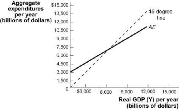
222.
(Figure: Aggregate Expenditures and Real GDP) Look at the figure Aggregate
Expenditures and Real GDP. At a real GDP of $9,000 billion:
A)
planned investment is less than actual investment.
B)
planned investment equals actual investment.
C)
planned investment is greater than actual investment.
D)
there will be no unplanned investment.
223.
(Figure: Aggregate Expenditures and Real GDP) Look at the figure Aggregate
Expenditures and Real GDP. If the level of real GDP equals $9,000 billion and there are
no changes in the consumption function or in planned investment, then real GDP will
_____in the next period.
A)
rise
B)
remain unchanged
C)
fall
D)
fall, but only if there is an offsetting change in autonomous consumption
224.
If aggregate expenditures are higher than real GDP:
A)
there are unplanned decreases in inventories.
B)
employment decreases.
C)
aggregate output decreases.
D)
actual real output is greater than equilibrium real output.
225.
If aggregate expenditures are lower than real GDP:
A)
there will be unplanned increases in inventories.
B)
employment increases.
C)
aggregate output increases.
D)
actual real output is less than equilibrium real output.
226.
If aggregate expenditures equal $800 billion and real GDP equals $600 billion:
A)
unplanned inventory accumulation equals $200 billion.
B)
unplanned inventory accumulation equals –$200 billion.
C)
consumption plus investment equals $200 billion.
D)
actual investment equals –$200 billion.
227.
If real GDP equals $700 billion and planned aggregate expenditures equal $400 billion:
A)
consumption plus planned investment equals $300 billion.
B)
actual investment equals –$300 billion.
C)
actual investment plus savings equals $300 billion.
D)
unplanned inventory accumulation equals $300 billion.
Page 45
228.
If real GDP exceeds aggregate expenditures, the economy will:
A)
contract, reducing employment.
B)
expand, causing inflation.
C)
expand, increasing employment.
D)
neither contract nor expand, holding employment constant.
229.
If aggregate expenditures exceed real GDP, the economy will:
A)
expand, increasing employment.
B)
expand, reducing prices.
C)
contract, decreasing employment.
D)
neither expand nor contract, holding employment the same.
Use the following to answer questions 230-231:
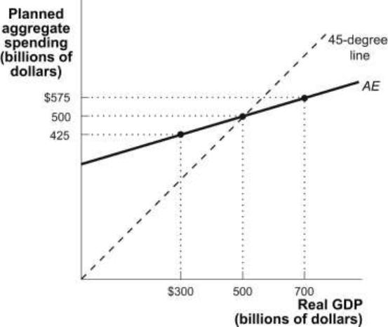
Figure: Aggregate Expenditures I
230.
(Figure: Aggregate Expenditures I) Look at the figure Aggregate Expenditures I. The
equilibrium real GDP is:
A)
$500 billion.
B)
$300 billion.
C)
$700 billion.
D)
$625 billion.
Page 46
231.
(Figure: Aggregate Expenditures I) Look at the figure Aggregate Expenditures I. When
real GDP is $700 billion, there will be a _____ in unplanned inventory investment.
A)
$125 million increase
B)
$125 million decline
C)
$200 million decline
D)
$200 million increase
232.
If real GDP is less than aggregate expenditure, then inventories will _____, and firms
will _____.
A)
increase; cut back on future production
B)
fall; increase the prices of their products
C)
increase; lower their product prices
D)
fall; increase their future production
233.
If real GDP is $1,000 billion and the aggregate expenditure is $850 billion, then the
change in inventories will be:
A)
–$150 million.
B)
$1,850 million.
C)
$150 million.
D)
–$1,850 million.
234.
When the economy is in income–expenditure equilibrium:
A)
exports equal imports.
B)
savings is less than investment spending.
C)
taxes equal transfer payments.
D)
real GDP equals planned aggregate spending.
235.
The Federal Reserve, the central bank of the United States, has been cutting the interest
rate to stimulate the recessionary economy. Interest cuts by the Federal Reserve are
supposed to:
A)
lower the savings rate in the economy and stop leakages.
B)
increase government spending on the economic infrastructure and thus increase
GDP through the multiplier process.
C)
increase cash holding by the general public, thus lowering their dependence on
credit.
D)
increase planned investment spending and thus increase GDP via the multiplier.
Page 47
236.
If the slope of the aggregate expenditures curve is 0.8, the multiplier is:
A)
1.
B)
4.
C)
5.
D)
infinity.
237.
If the slope of the aggregate expenditures curve is 0.9, the multiplier is:
A)
1.
B)
4.
C)
5.
D)
10.
238.
If the slope of the aggregate expenditures curve is 0.75, the multiplier is:
A)
1.
B)
4.
C)
5.
D)
infinity.
239.
The magnitude of the multiplier process that links planned aggregate spending to real
GDP is determined by:
A)
the marginal propensity to save.
B)
the interest rate.
C)
the level of autonomous consumption.
D)
the level of planned investment spending.
240.
If planned aggregate spending rises by $10 billion and the marginal propensity to
consume is 0.75, then equilibrium real GDP changes by:
A)
$2.5 billion.
B)
$7.5 billion.
C)
$10 billion.
D)
$40 billion.
241.
If planned aggregate spending rises by $25 billion and the marginal propensity to
consume is 0.8, then equilibrium real GDP changes by:
A)
$25 billion.
B)
$125 billion.
C)
$200 billion.
D)
$250 billion.
Page 48
242.
An autonomous increase in aggregate spending _____ real GDP by _____.
A)
reduces; that amount
B)
increases; that amount
C)
reduces; more than that amount
D)
increases; more than that amount
243.
The primary cause of the recession that ended in late 2001 was:
A)
a slump in business investment spending.
B)
too much investment spending by households, crowding out business investment
spending.
C)
an increase in income tax rates.
D)
a decrease in government spending.
244.
The recession began to wind down in late 2001 mainly because of an increase in:
A)
tax rates on capital gains.
B)
consumer spending on durable goods, especially automobiles.
C)
consumer spending on nondurables, especially gasoline and clothing.
D)
consumer savings.
245.
In the last quarter of 2001, when consumer spending was ending the recession, GDP
growth was slow at first because:
A)
consumer savings also decreased.
B)
tax rates increased.
C)
inventories, which had built up during the recession, decreased.
D)
inventories of consumer goods increased.
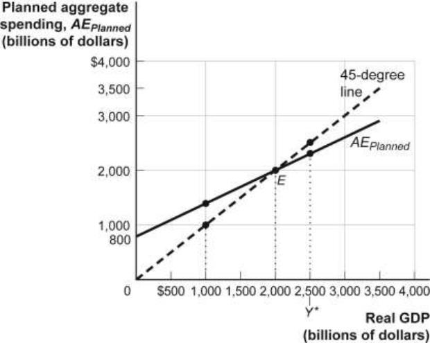
Use the following to answer questions 246-254:
Scenario: Income–Expenditure Equilibrium
Real GDP is $8,000, autonomous consumption is $500, and planned investment spending is
$200. The marginal propensity to consume is 0.8.
246.
(Scenario: Income–Expenditure Equilibrium) Look at the scenario Income–Expenditure
Equilibrium. What is the consumption function?
A)
C = 8,000 + 0.8 × YD
B)
C = 8,700 + 0.2 × YD
C)
C = 500 + 0.8 × YD
D)
C = 1,700 + 0.2 × YD
Page 49
247.
(Scenario: Income–Expenditure Equilibrium) Look at the scenario Income–Expenditure
Equilibrium. How much is consumption?
A)
$500
B)
$8,000
C)
$700
D)
$6,900
248.
(Scenario: Income–Expenditure Equilibrium) Look at the scenario Income–Expenditure
Equilibrium. How much is planned aggregate spending?
A)
$7,100
B)
$6,400
C)
$8,000
D)
$700
249.
(Scenario: Income–Expenditure Equilibrium) Look at the scenario Income–Expenditure
Equilibrium. How much is unplanned inventory investment?
A)
$1,100
B)
–$900
C)
$900
D)
0
250.
(Scenario: Income–Expenditure Equilibrium) Look at the scenario Income–Expenditure
Equilibrium. Given this income–expenditure equilibrium, firms will tend to:
A)
raise prices.
B)
hire more people.
C)
increase output.
D)
decrease output.
251.
(Scenario: Income–Expenditure Equilibrium) Look at the scenario Income–Expenditure
Equilibrium. If real GDP is $3,000, planned aggregate spending is:
A)
$2,400.
B)
$2,900.
C)
$3,100.
D)
$3,000.

Page 50
252.
(Scenario: Income–Expenditure Equilibrium) Look at the scenario Income–Expenditure
Equilibrium. If real GDP is $3,000, how much is unplanned inventory investment?
A)
0
B)
$600
C)
$100
D)
–$100
253.
(Scenario: Income–Expenditure Equilibrium) Look at the scenario Income–Expenditure
Equilibrium. Income–expenditure equilibrium is achieved when GDP is:
A)
$8,000.
B)
$7,000.
C)
$3,500.
D)
$700.
254.
(Scenario: Income–Expenditure Equilibrium) Look at the scenario Income–Expenditure
Equilibrium. The multiplier is:
A)
0.8.
B)
0.2.
C)
5.
D)
1.25.
Use the following to answer questions 255-258:
Table: The Economy of Albernia
Real GDP
(in billions)
Disposable Income
(in billions)
Consumption
(in billions)
Planned Investment
(in billions)
$ 0
$ 0
$ 400
$600
500
500
700
600
1,000
1,000
1,000
600
1,500
1,500
1,300
600
2,000
2,000
1,600
600
2,500
2,500
1,900
600
3,000
3,000
2,200
600
Page 51
255.
(Table: The Economy of Albernia) Look at the table The Economy of Albernia. What is
the consumption function for Albernia?
A)
C = 600 + 0.3 × YD
B)
C = 600 + 0.75 × YD
C)
C = 400 + 0.6 × YD
D)
C = 400 + 0.75 × YD
256.
(Table: The Economy of Albernia) Look at the table The Economy of Albernia. What is
the income–expenditure equilibrium real GDP?
A)
$1,000 billion
B)
$1,500 billion
C)
$2,000 billion
D)
$2,500 billion
257.
(Table: The Economy of Albernia) Look at the table The Economy of Albernia. If real
GDP is $1,500 billion, then the level of unplanned inventories is:
A)
$400 billion.
B)
–$400 billion.
C)
$600 billion.
D)
–$600 billion.
258.
(Table: The Economy of Albernia) Look at the table The Economy of Albernia. If real
GDP is $3,000 billion, then unplanned investment is:
A)
zero.
B)
$100 billion.
C)
$200 billion.
D)
$300 billion.
Page 52
Use the following to answer questions 259-262:
Figure: Income–Expenditure Equilibrium
259.
(Figure: Income–Expenditure Equilibrium) Look at the table Income–Expenditure
Equilibrium. If planned investment spending increases in this economy:
A)
aggregate expenditures curve will shift up, increasing the income–expenditure
equilibrium.
B)
aggregate expenditures curve will shift down, decreasing the income–expenditure
equilibrium.
C)
economy will move upward along the aggregate expenditures curve, increasing the
income–expenditure equilibrium.
D)
economy will move downward along the aggregate expenditures curve, decreasing
the income–expenditure equilibrium.
260.
(Figure: Income–Expenditure Equilibrium) Look at the table Income–Expenditure
Equilibrium. If investment spending decreases in this economy, then the:
A)
aggregate expenditures curve will shift up, increasing the income–expenditure
equilibrium.
B)
aggregate expenditures curve will shift down, decreasing the income–expenditure
equilibrium.
C)
economy will move upward along the aggregate expenditures curve, increasing the
income–expenditure equilibrium.
D)
economy will move downward along the aggregate expenditures curve, decreasing
the income–expenditure equilibrium.

Page 53
261.
(Figure: Income–Expenditure Equilibrium) Look at the table Income–Expenditure
Equilibrium. If planned investment spending increases autonomously by $100, real GDP
will:
A)
increase by $250.
B)
increase by $100.
C)
increase by $125.
D)
not change.
262.
(Figure: Income–Expenditure Equilibrium) Look at the table Income–Expenditure
Equilibrium. If planned investment spending increases by $100, income–expenditure
equilibrium occurs at real GDP of:
A)
$8,100.
B)
$3,600
C)
$2,250.
D)
$4,000.
Use the following to answer questions 263-265:
263.
(Table: Aggregate Spending) Look at the table Aggregate Spending. Suppose the
economy has no government spending and no foreign trade. With no taxes or transfers,
real GDP equals disposable income (YD). At what level of real GDP will the economy
find its income–expenditure equilibrium?
A)
$2,000
B)
$2,500
C)
$3,500
D)
$4,500
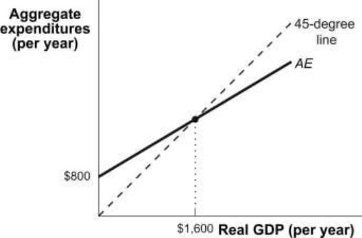
Page 54
264.
(Table: Aggregate Spending) Look at the table Aggregate Spending. Suppose the
economy has no government spending and no foreign trade. With no taxes or transfers,
real GDP equals disposable income (YD). If real GDP is $2,500, what is the level of
unplanned inventory investment?
A)
$200
B)
$0
C)
$2,700
D)
–$200
265.
(Table: Aggregate Spending) Look at the table Aggregate Spending. Suppose the
economy has no government spending and no foreign trade. With no taxes or transfers,
real GDP equals disposable income (YD). The income–expenditure equilibrium real
GDP is found at _____. If planned investment fell to $300, the new income–expenditure
equilibrium real GDP would fall to _____.
A)
$3,500; $2,500
B)
$3,500; $2,000
C)
$3,000; $1,500
D)
$4,000; $2,500
Use the following to answer questions 266-271:
Figure: Aggregate Expenditures Curve I
Page 55
266.
(Figure: Aggregate Expenditures Curve I) Look at the figure Aggregate Expenditures
Curve I. The equilibrium level of real GDP in the aggregate expenditures model shown
in this figure is:
A)
$800.
B)
$1,000.
C)
$1,600.
D)
$3,200.
267.
(Figure: Aggregate Expenditures Curve I) Look at the figure Aggregate Expenditures
Curve I. The slope of the aggregate expenditures curve in this figure is:
A)
0.25.
B)
0.5.
C)
1.0.
D)
45 degrees.
268.
(Figure: Aggregate Expenditures Curve I) Look at the figure Aggregate Expenditures
Curve I. The multiplier in the aggregate expenditures model shown in this figure is:
A)
1.
B)
2.
C)
3.
D)
5.
269.
(Figure: Aggregate Expenditures Curve I) Look at the figure Aggregate Expenditures
Curve I. Suppose that the consumption function in this economy rises by $100. The
result would be a shift in the aggregate expenditures curve:
A)
upward by $100.
B)
upward by $200.
C)
upward by $100 times the multiplier.
D)
downward by $200.
270.
(Figure: Aggregate Expenditures Curve I) Look at the figure Aggregate Expenditures
Curve I. Suppose that the consumption function in this economy rises by $100. The
result will be a _____ increase in the equilibrium level of real GDP.
A)
$100.
B)
$200.
C)
$800.
D)
$1,600.

Page 56
271.
(Figure: Aggregate Expenditures Curve I) Look at the figure Aggregate Expenditures
Curve I. Suppose that the government’s purchases of goods and services in this economy
rise by $100. Real GDP will:
A)
decrease by $100.
B)
increase by $200.
C)
increase by $800.
D)
decrease by $200.
Use the following to answer questions 272-277:
Figure: Aggregate Expenditures Curve II
272.
(Figure: Aggregate Expenditures Curve II) Look at the table Aggregate Expenditures
Curve II. The equilibrium level of real GDP in the aggregate expenditures model shown
in this figure is:
A)
$800.
B)
$1,000.
C)
$2,000.
D)
$4,000.
273.
(Figure: Aggregate Expenditures Curve II) Look at the table Aggregate Expenditures
Curve II. The slope of the aggregate expenditures curve is:
A)
0.25.
B)
0.5.
C)
0.6.
D)
45 degrees.
Page 57
274.
(Figure: Aggregate Expenditures Curve II) Look at the table Aggregate Expenditures
Curve II. The multiplier is:
A)
1.0.
B)
2.0.
C)
2.5.
D)
5.0.
275.
(Figure: Aggregate Expenditures Curve II) Look at the table Aggregate Expenditures
Curve II. Suppose that the consumption function in this figure rises by $100. The
aggregate expenditures curve would shift upward by:
A)
$100.
B)
$250.
C)
$100 times the multiplier.
D)
$150.
276.
(Figure: Aggregate Expenditures Curve II) Look at the table Aggregate Expenditures
Curve II. Suppose that the consumption function rises by $100. The equilibrium level of
real GDP would rise by:
A)
$100.
B)
$200.
C)
$250.
D)
$50.
277.
(Figure: Aggregate Expenditures Curve II) Look at the table Aggregate Expenditures
Curve II. Suppose that the consumption function in this economy rises by $200.
Equilibrium real GDP would rise by:
A)
$100.
B)
$200.
C)
$250.
D)
$500.

Page 58
Use the following to answer questions 278-279:
Figure: Aggregate Expenditures Curve III
278.
(Figure: Aggregate Expenditures Curve III) Look at the table Aggregate Expenditures
Curve III. Suppose that the consumption function in this figure rises by $100. The
aggregate expenditures curve will shift upward by:
A)
$100.
B)
$400.
C)
$100 times the multiplier.
D)
$200 times the multiplier.
279.
(Figure: Aggregate Expenditures Curve III) Look at the table Aggregate Expenditures
Curve III. Suppose that the consumption function shifts upward by $100. Equilibrium
real GDP will rise by:
A)
$100.
B)
$400.
C)
$800.
D)
$3,200.
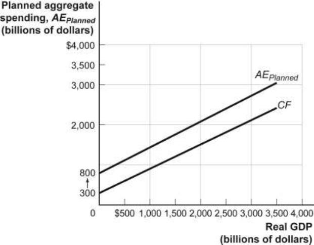
Page 59
Use the following to answer questions 280-285:
Figure: The Aggregate Consumption Function and Planned Aggregate Spending
280.
(Figure: The Aggregate Consumption Function and Planned Aggregate Spending) Look
at the table The Aggregate Consumption Function and Planned Aggregate Spending. If
current disposable income increases in this economy, then the:
A)
aggregate expenditures curve will shift up.
B)
aggregate expenditures curve will shift down.
C)
economy will move upward along the aggregate expenditures curve.
D)
economy will move downward along the aggregate expenditures curve.
281.
(Figure: The Aggregate Consumption Function and Planned Aggregate Spending) Look
at the table The Aggregate Consumption Function and Planned Aggregate Spending. If
disposable income decreases, then the:
A)
aggregate expenditures curve will shift up.
B)
aggregate expenditures curve will shift down.
C)
economy will move upward along the aggregate expenditures curve.
D)
economy will move downward along the aggregate expenditures curve.
Page 60
282.
(Figure: The Aggregate Consumption Function and Planned Aggregate Spending) Look
at the table The Aggregate Consumption Function and Planned Aggregate Spending. If
expected disposable income increases, then the:
A)
aggregate expenditures curve will shift up.
B)
aggregate expenditures curve will shift down.
C)
economy will move upward along the aggregate expenditures curve.
D)
economy will move downward along the aggregate expenditures curve.
283.
(Figure: The Aggregate Consumption Function and Planned Aggregate Spending) Look
at the table The Aggregate Consumption Function and Planned Aggregate Spending. If
expected disposable income decreases in this economy, then the:
A)
aggregate expenditures curve will shift up.
B)
aggregate expenditures curve will shift down.
C)
economy will move upward along the aggregate expenditures curve.
D)
economy will move downward along the aggregate expenditures curve.
284.
(Figure: The Aggregate Consumption Function and Planned Aggregate Spending) Look
at the table The Aggregate Consumption Function and Planned Aggregate Spending. If
aggregate wealth increases, the:
A)
aggregate expenditures curve will shift up.
B)
aggregate expenditures curve will shift down.
C)
economy will move upward along the aggregate expenditures curve.
D)
economy will move downward along the aggregate expenditures curve.
285.
(Figure: The Aggregate Consumption Function and Planned Aggregate Spending) Look
at the table The Aggregate Consumption Function and Planned Aggregate Spending. If
aggregate wealth decreases, then the:
A)
aggregate expenditures curve will shift up.
B)
aggregate expenditures curve will shift down.
C)
economy will move upward along the aggregate expenditures curve.
D)
economy will move downward along the aggregate expenditures curve.
286.
Between 2003 and 2010, the unemployment rate in Ft. Myers, Florida, decreased from
13% to 3%.
A)
True
B)
False
Page 61
287.
Much of the housing boom in Ft. Myers was due to speculators who bought homes not
to live in themselves but to resell quickly at much higher prices.
A)
True
B)
False
288.
The changes in the economy of Ft. Myers between 2003 and 2010 illustrate that the
multiplier has positive effects but not negative effects.
A)
True
B)
False
289.
The housing market in Ft. Myers collapsed in the mid to late 2000s because of extensive
damage to homes from hurricanes.
A)
True
B)
False
290.
The expansion and collapse of the housing market in Ft. Myers between 2003 and 2010
is primarily an example of how changes in investment spending can affect consumer
spending and the entire economy.
A)
True
B)
False
291.
The marginal propensity to consume is the increase in consumer spending when
disposable income increases by $1.
A)
True
B)
False
292.
The marginal propensity to save is the increase in household savings when investment
spending increases by $1.
A)
True
B)
False
293.
In a simple economy with no taxes, government spending, exports, or imports, any
disposable income that is not consumed is saved.
A)
True
B)
False
Page 62
294.
In a simple economy with no taxes, government spending, exports, or imports, if
disposable income increases by $500 and $450 is consumed, $950 is saved.
A)
True
B)
False
295.
In a simple economy with no taxes, government spending, exports, or imports, if
disposable income increases by $500 and $450 is consumed, $50 is saved.
A)
True
B)
False
296.
A $200 million increase in investment spending will increase real GDP by exactly $200
million.
A)
True
B)
False
297.
A $200 million increase in investment spending will increase real GDP by more than
$200 million.
A)
True
B)
False
298.
A $300 million decrease in investment spending will increase real GDP by more than
$300 million.
A)
True
B)
False
299.
A $600 million decrease in investment spending will decrease real GDP by more than
$600 million.
A)
True
B)
False
300.
Autonomous spending occurs in the second round of spending increases caused by the
multiplier.
A)
True
B)
False
Page 63
301.
Autonomous spending is an initial change in the desired level of spending by firms,
households, or government at a given level of real GDP.
A)
True
B)
False
302.
If the marginal propensity to save is 0.25 in an economy with no taxes and no imports,
the marginal propensity to consume is 1.25.
A)
True
B)
False
303.
If the marginal propensity to save is 0.25 in an economy with no taxes and no imports,
the marginal propensity to consume is 0.75.
A)
True
B)
False
304.
In an economy with no taxes or imports, if the marginal propensity to consume
increases, the marginal propensity to save will also increase.
A)
True
B)
False
305.
In an economy with no taxes or imports, if the marginal propensity to consume
increases, the marginal propensity to save will decrease.
A)
True
B)
False
306.
In an economy with no taxes or imports, if disposable income increases by $2,000 and
consumption increases by $1,400, the marginal propensity to save is 0.21.
A)
True
B)
False
307.
In an economy with no taxes or imports, if disposable income decreases by $2,000 and
consumption decreases by $1,400, the marginal propensity to save is 0.3.
A)
True
B)
False
Page 64
308.
In an economy with no taxes or imports, if disposable income decreases by $2,000 and
consumption decreases by $1,400, the multiplier is 7.
A)
True
B)
False
309.
In an economy with no taxes or imports, if disposable income decreases by $2,000 and
consumption decreases by $1,500, the marginal propensity to consume is –0.25.
A)
True
B)
False
310.
In an economy with no taxes or imports, if disposable income decreases by $2,000 and
consumption decreases by $1,500, the multiplier is –4.
A)
True
B)
False
311.
In an economy with no taxes and no imports, disposable income increases from $1,000
to $2,000. If consumption increases from $800 to $1500, the marginal propensity to
consume is 0.7.
A)
True
B)
False
312.
In an economy with no taxes and no imports, disposable income increases from $1,000
to $2,000. If consumption increases from $800 to $1,500, the marginal propensity to
save is 0.25.
A)
True
B)
False
313.
In an economy with no taxes and no imports, disposable income increases from $1,000
to $2,000. If consumption increases from $800 to $1,500, the marginal propensity to
save is 0.3.
A)
True
B)
False
314.
In an economy with no taxes and no imports, disposable income increases from $1,000
to $2,000. If consumption increases from $800 to $1,500, the multiplier is 3.33.
A)
True
B)
False
Page 65
315.
If the marginal propensity to consume decreases, the multiplier will increase.
A)
True
B)
False
316.
If the marginal propensity to save decreases, the multiplier will increase.
A)
True
B)
False
317.
If the marginal propensity to consume is 0.9, the multiplier will be 0.1.
A)
True
B)
False
318.
If the marginal propensity to save is 0.2, the multiplier will be 5.
A)
True
B)
False
319.
If the marginal propensity to consume is 0.9 and investment spending increases by $50
billion, the change in real GDP will be $5 billion.
A)
True
B)
False
320.
If the marginal propensity to save is 0.25 and investment spending increases by $50
billion, the change in real GDP will be $200 billion.
A)
True
B)
False
321.
If the consumption function is C = $100 million + 0.8 × YD, then the marginal
propensity to consume is $100 million.
A)
True
B)
False
322.
The marginal propensity to consume is consumption divided by disposable income.
A)
True
B)
False
Page 66
323.
If you expect to get a substantial raise six months from now and if you are like most
people, it will not affect your current consumption because you haven’t received the
money yet.
A)
True
B)
False
324.
The aggregate consumption function can shift because of changes in expected
disposable income and in aggregate wealth.
A)
True
B)
False
325.
According to the life-cycle hypothesis, consumers plan their spending based on their
current disposable income when they are very young.
A)
True
B)
False
326.
People use wealth to smooth consumption over their life cycle.
A)
True
B)
False
327.
Planned investment spending is inversely related to the interest rate, because fewer
projects are profitable at higher interest rates.
A)
True
B)
False
328.
If expected GDP increases, then current planned investment will increase.
A)
True
B)
False
329.
The higher current production capacity is, the higher current planned investment will be.
A)
True
B)
False
330.
Planned investment spending and actual investment spending are NOT always equal.
A)
True
B)
False
Page 67
331.
If planned investment is $50 billion and unplanned inventory investment is $10 billion,
then actual investment is $40 billion.
A)
True
B)
False
332.
Inventories are counted as investment because inventories are a source of future sales.
A)
True
B)
False
333.
If real GDP is greater than planned expenditure, unplanned inventory investment is
negative.
A)
True
B)
False
334.
Changes in unplanned inventory investment move the economy toward the
income–expenditure equilibrium.
A)
True
B)
False
335.
Decreases in investment spending are usually offset by increases in consumption
through the multiplier process.
A)
True
B)
False
336.
If planned aggregate spending rises by $10 billion and the marginal propensity to
consume is 0.8, then the income–expenditure equilibrium increases by 50 billion.
A)
True
B)
False
337.
If planned aggregate spending rises by $20 billion and the marginal propensity to
consume is 0.9, then the income–expenditure equilibrium increases by $18 billion.
A)
True
B)
False
338.
The main cause of the recession that ended in late 2001 was a decrease in consumer
savings.
A)
True
B)
False

Page 68
339.
An increase in consumer spending on durable goods was the main factor that ended the
recession in 2001.
A)
True
B)
False
340.
Negative inventory investment caused the growth of GDP to be fairly low when the
recovery from the recession began in the fourth quarter of 2001.
A)
True
B)
False
341.
Explain how the boom and bust in the Ft. Myers housing market between 2003 and
2010 illustrates the positive and negative effects of the multiplier.
342.
Suppose that the marginal propensity to consume is 0.80 and the government spends
$10 million to repair a bridge. Assuming no taxes and no international trade, explain
how the $10 million of government spending will increase GDP by $50 million.
343.
How does a nation’s savings rate, as measured by the marginal propensity to save, affect
the size of the spending multiplier?
344.
How can autonomous consumption be greater than zero when disposable income equals
zero?
345.
Suppose you have estimated the consumption function as C = 250 + 0.90 × YD. What is
the equation for the corresponding savings function?
Use the following to answer question 346:
Table: Consumption for Four Consumers
Disposable Income
Brandy’s
Consumption
Mandy’s
Consumption
Sandy’s
Consumption
Candi’s
Consumption
$ 0
$ 500
$1,000
$ 800
$1,200
1,000
1,000
1,900
1,600
1,800
2,000
1,500
2,800
2,400
2,400
3,000
2,000
3,700
3,200
3,000
4,000
2,500
4,600
4,000
3,600
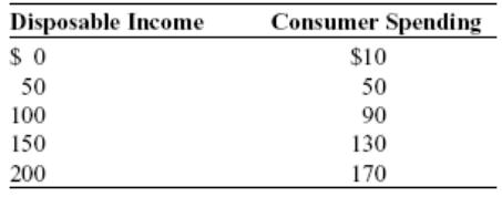
Page 69
346.
(Table: Consumption for Four Consumers) Look at the table Consumption for Four
Consumers. Construct the aggregate consumption function.
347.
Suppose the economy is in income–expenditure equilibrium. How will each of the
following situations affect planned investment and unplanned inventory investment?
a. The Federal Reserve decreases interest rates.
b. Major economic indicators decrease business optimism about growth in real GDP.
348.
In a simple economy with no government and no foreign sector, autonomous consumer
spending is $100 and planned investment spending is $300. The marginal propensity to
consume is 0.75.
a. Solve for the equilibrium level of real GDP.
b. If real GDP is $2,000, what is unplanned inventory investment?
349.
In a simple economy with no government and no foreign sector, autonomous consumer
spending is $250 and planned investment spending is $500. The marginal propensity to
consume is 0.80.
a. Solve for the equilibrium level of real GDP.
b. Suppose that interest rates fall and planned investment increases by $100. What is the
new level of equilibrium real GDP?
Use the following to answer questions 350-351:
Table: Disposable Income and Spending
350.
(Table: Disposable Income and Spending) Look at the table Disposable Income and
Spending. Calculate the marginal propensity to consume (MPC). Use this MPC to
compute the spending multiplier.
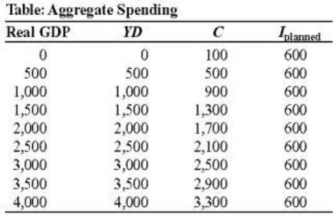
Page 70
351.
(Table: Disposable Income and Spending) Look at the table Disposable Income and
Spending. Develop a linear equation of the consumption function. Use this consumption
function to forecast the amount of consumption spending that would occur if disposable
income were equal to $500.
Use the following to answer question 352:
352.
(Table: Real GDP) Suppose the economy has no government spending and no foreign
trade. With no taxes and transfers, real GDP equals disposable income (YD). The data in
the accompanying table show consumption spending (C) and planned investment
(IPlanned).
a. What is the marginal propensity to consume in this economy?
b. At what level of real GDP will the economy find its income–expenditure equilibrium?
353.
The multiplier process:
A)
explains how spending continues indefinitely with continuous rounds of spending.
B)
ends after one round of spending and with total spending limited to the initial
change in spending.
C)
occurs only when economies are in an expansion phase.
D)
is limited, with the total change in real GDP dependent upon the size of the
marginal propensity to consume.
354.
The value of the multiplier will be smaller:
A)
the larger the value of the marginal propensity to save.
B)
the larger the value of the marginal propensity to consume.
C)
if the marginal propensity to consume equals the marginal propensity to save.
D)
if the marginal propensity to consume plus the marginal propensity to save equals
1.
Page 71
355.
During the Great Depression:
A)
investment fell, but consumption increased.
B)
investment increased, but consumption decreased.
C)
both consumption and investment decreased.
D)
overall GDP rose.
356.
All of the following affect consumer spending EXCEPT:
A)
current disposable income.
B)
wealth.
C)
past disposable income.
D)
expected disposable income.
357.
Two-thirds of total spending is usually attributed to:
A)
consumption.
B)
investment.
C)
government spending.
D)
net exports.
358.
The marginal propensity to save:
A)
is the change in consumer savings divided by the change in consumption.
B)
is the change in savings divided by the change in disposable income.
C)
equals MPC + 1.
D)
changes when the marginal propensity to consume is constant.
359.
Alice’s disposable income increases by $1,000, and she spends $600 of it. Assuming no
taxes, Alice’s:
A)
marginal propensity to save is 0.4 and she saves $400.
B)
MPC is 0.4 and she saves $400.
C)
marginal propensity to save is 0.4 and she saves $600.
D)
MPC is 0.6 and she consumes $400.
360.
When Julie Ann’s disposable income is $10,000, she spends $10,000, and when her
disposable income is $15,000, her spending is $12,500. Julie Ann’s autonomous
consumption is _____ and her marginal propensity to consume is 0.5.
A)
$5,000
B)
$10,000
C)
$15,000
D)
$0
Page 72
361.
The slope of the consumption function equals:
A)
1 – MPS.
B)
1 / (1 – MPS).
C)
1 – MPC.
D)
MPC / MPS.
362.
If housing prices rise nationwide, there will be a(n):
A)
increase in consumer spending at any given level of disposable income.
B)
decrease in wealth as consumers spend more income on mortgage payments.
C)
decrease in overall aggregate expenditures.
D)
drop in investment spending.
363.
A decrease in consumer spending is likely to be caused by:
A)
expectation of an increase in personal income taxes.
B)
expectation of a decrease in personal income taxes.
C)
an increase in the multiplier.
D)
an increase in investment spending.
364.
When consumers receive more disposable income, their spending:
A)
will increase.
B)
will decrease.
C)
will stay the same, but their savings will decrease.
D)
and their savings will both decrease.
365.
The permanent income hypothesis suggests that consumer:
A)
spending depends on income people expect over the long term rather than on
current income.
B)
spending is smoothed each month in response to changes in their current disposable
income.
C)
spending is made up of an autonomous amount and an amount dependent upon
disposable income.
D)
savings depends on one’s lifetime income.
366.
Vanessa tells people she is consuming more now and probably will continue to do so for
some time, but she believes her consumption will smooth out over her lifetime.
Vanessa’s consumption pattern mirrors the _____:
A)
multiplier hypothesis.
B)
life-cycle income hypothesis.
C)
relative income hypothesis.
D)
accelerator principle.
Page 73
Use the following to answer questions 367-368:
Scenario: Aggregate Consumption Function
Suppose the aggregate consumption function is given by C = 1,000 + 0.75YD, where C is
consumption and YD is disposable income.
367.
(Scenario: Aggregate Consumption Function) Look at the scenario Aggregate
Consumption Function. If disposable income increases by $100, aggregate consumption
will increase by _____ and autonomous consumption _____.
A)
$75; remains at $1,000
B)
$1000; remains at $75
C)
$100; increases by $100
D)
$175; increases by $100
368.
(Scenario: Aggregate Consumption Function) Look at the scenario Aggregate
Consumption Function. If aggregate disposable income equals $1,000, then aggregate
consumption equals:
A)
$1,000.
B)
$1,750.
C)
$2,000.
D)
$1,075.
369.
Interest rates and planned investment spending:
A)
have a positive relationship.
B)
exhibit a negative relationship.
C)
have no relationship, since planned investment is fixed.
D)
have no relationship if the firm has retained earnings.
370.
A firm has enough retained earnings to finance an investment project. For this firm, the
market interest rate:
A)
is not relevant to the investment decision.
B)
indicates the opportunity cost of using retained earnings.
C)
will help to calculate the rate of return for the project.
D)
has no impact on the profitability of the investment project.
Page 74
371.
The belief that a higher rate of growth in real GDP will lead to higher planned
investment spending is known as:
A)
the accelerator principle.
B)
the multiplier effect.
C)
fiscal policy with an emphasis on government spending.
D)
unplanned investment spending.
372.
Planned investment spending is:
A)
investment that firms intend to make during a given period.
B)
inventory investment changes.
C)
not considered part of GDP.
D)
dependent only on interest rates.
373.
The multiplier process assumes that:
A)
aggregate prices are perfectly flexible.
B)
the economy is open and there is free trade.
C)
the economy is operating with sticky aggregate price levels.
D)
interest rates are constantly changing.
374.
Suppose the level of planned aggregate expenditure in an economy is $1,000 and real
GDP is $800. According to the simple model developed in this chapter, in which the
aggregate price level is assumed to be constant, we can expect:
A)
inventories to stay the same, since this is part of planned investment.
B)
inventories to decrease.
C)
inventories to increase.
D)
real GDP to fall further.
375.
If unplanned inventory investment is positive, probably:
A)
the economy is growing rapidly.
B)
aggregate expenditures on goods and services are less than forecast.
C)
the economy is doing the same, since inventory changes do not affect the economy.
D)
the stock of inventories is declining.
376.
In the income–expenditure model, inventories are:
A)
fixed and therefore provide little insight into the direction of the economy.
B)
a long-run event that aids forecasters in understanding where long-run real GDP is.
C)
constantly changing and provide insight into the future of the economy.
D)
often positive, suggesting that additions to inventory stocks are a long-run goal.
Page 75
377.
If the marginal propensity to consume equals 0.75, then based on the simple model
presented in this chapter, one would expect a $100 decrease in investment spending to
lead to a total _____ in spending of _____.
A)
increase; $100.
B)
increase; $400.
C)
decrease; $100.
D)
decrease; $400.
Use the following to answer questions 378-382:
Scenario: A Country’s Consumption Function
A country is closed. It has no government sector, and its aggregate price levels and interest rates
are fixed. Furthermore, the marginal propensity to consume is constant and the country’s
consumption function is as follows: C = 200 + 0.75YD, where YD is disposable income and C is
consumption. Assume that planned investment equals 75.
378.
(Scenario: A Country’s Consumption Function) Look at the scenario A Country’s
Consumption Function. If this country’s income increased by $10,000, consumption
would increase by:
A)
$10,000.
B)
$7,500.
C)
$200.
D)
$7,700.
379.
(Scenario: A Country’s Consumption Function) Look at the scenario A Country’s
Consumption Function. When real GDP equals $900:
A)
planned investment equals $900.
B)
unplanned inventory investment is negative.
C)
autonomous consumption equals $900.
D)
the economy is in income–expenditure equilibrium.
380.
(Scenario: A Country’s Consumption Function) Look at the scenario A Country’s
Consumption Function. What is the income–expenditure equilibrium for this country?
A)
$900
B)
$1,100
C)
$275
D)
$200
Page 76
381.
(Scenario: A Country’s Consumption Function) Look at the scenario A Country’s
Consumption Function. Holding everything else constant, what will happen if aggregate
wealth decreases by $100?
A)
The aggregate expenditures curve will shift downward.
B)
The income–expenditure equilibrium real GDP will increase by more than $100.
C)
There will be no multiplier effect on real GDP, since there is a drop in aggregate
wealth.
D)
Planned investment will increase.
382.
(Scenario: A Country’s Consumption Function) Look at the scenario A Country’s
Consumption Function. If real GDP is $1,100:
A)
unplanned investment equals zero.
B)
planned investment equals zero.
C)
the aggregate expenditures curve shifts up.
D)
the marginal propensity to consume decreases.

Page 77
Answer Key

Page 78

Page 79

Page 80

Page 81

Page 82

Page 83

Page 84
Page 85

Page 86