
Managerial Decision Modeling w/ Spreadsheets, 3e (Balakrishnan/Render/Stair)
Chapter 11 Forecasting Models
11.1 Chapter Questions
1) Consider the following data that was fitted using a Linear Trend.
Period
Actual value
(or) Y
Period number
(or) X
Period 1
10
1
Period 2
11
2
Period 3
9
3
Period 4
12
4
Period 5
13
5
Period 6
12
6
Period 7
15
7
The intercept of the trend line is 8.714, and the slope is 0.75. What is the forecast for period 8?
A) 13.714
B) 14.714
C) 15.714
D) 16.714
E) 15.75
2) Which of the following is considered to be a category of forecasting models?
A) Qualitative
B) Time-series
C) Causal models
D) both A and B
E) A, B, and C

3) Which of the following is NOT a qualitative method of forecasting?
A) Delphi Method
B) Trend Analysis
C) Jury of Executive Opinion
D) Sales Force Composition
E) Consumer Market Survey
4) Which of the following is NOT considered to be a Time-Series method of forecasting?
A) Simple Linear Regression
B) Moving Average
C) Exponential Smoothing
D) Seasonality Analysis
E) Multiplicative/Additive Decomposition
5) An iterative group process that allows experts, who may be located in different places, to make
forecasts is referred to as ________.
A) a jury of executive opinion
B) a sales force composite
C) ca onsumer market survey
D) the Delphi method
E) trend analysis

6) Consider the following data that was fitted using a linear trend.
Period
Actual value
(or) Y
Period number
(or) X
Period 1
10
1
Period 2
11
2
Period 3
9
3
Period 4
12
4
Period 5
13
5
Period 6
12
6
Period 7
15
7
The intercept of the trend line is 8.714, and the slope is 0.75. What is the forecast error for period 7?
A) 1.036
B) 8
C) 2.37
D) 5.714
E) 4.75

7) Consider the following data and Excel output for a simple linear regression model. How much of the
total variation in the dependent variable (Y) is explained by the independent variable (X)?
Period
Y
X
Period 1
10
1
Period 2
11
2
Period 3
9
3
Period 4
12
4
Period 5
13
5
Period 6
12
6
Period 7
15
7
Intercept
2.267
Slope
0.843
SE
1.810
Correlation
0.890
r-squared
0.791
A) 2.267
B) 0.843
C) 1.810
D) 0.890
E) 0.791

8) Consider the following data and its associated Excel output for a simple linear regression model.
How would you describe the linear relationship between Y and X?
Period
Y
X
Period 1
10
1
Period 2
11
2
Period 3
9
3
Period 4
12
4
Period 5
13
5
Period 6
12
6
Period 7
15
7
Intercept
2.267
Slope
0.843
SE
1.810
Correlation
0.890
r-squared
0.791
A) no relationship
B) positive relationship
C) negative relationship
D) inverse relationship
E) not enough information is provided
9) The value of the coefficient of determination R2 ranges between
A) 0 and -1
B) -1 and +1
C) 0 and +1
D) – infinity and + infinity
E) +1 and + infinity

10) The value of the correlation coefficient “r” ranges between
A) – infinity and + infinity
B) +1 and + infinity
C) 0 and -1
D) -1 and +1
E) 0 and +1
11) “Blips” in the data that follow no discernible pattern are referred to as
A) trend
B) random variations
C) seasonality
D) cycles
E) stationary variations
12) Consider the following forecast errors. What is the Mean Absolute Deviation (MAD)?
Period
Error
1
-2
2
1
3
3
4
0
5
-1
6
2
7
4
A) 1
B) 1.86
C) 7
D) 13
E) 5

13) Consider the following time series data. Suppose that you use exponential smoothing with an alpha
of 0.7 to fit a forecasting model. The forecast for period 7 is
Period
Forecast
Actual value
Period 1
10
10
Period 2
10
11
Period 3
10.7
9
Period 4
9.51
12
Period 5
11.253
13
Period 6
12.476
11
A) 10.443
B) 12
C) 9.443
D) 12.443
E) 11.443
14) The least squares method for linear regression:
A) minimizes the sum of the errors
B) minimizes the sum of the squared errors
C) maximizes forecasting accuracy
D) minimizes the value of the coefficient of determination R2
E) minimizes the regression equation coefficients
15) Suppose that you intend to use Solver to compute the optimal weights for a weighted moving
average. Changing variable cells would refer to:
A) the MAD cell
B) the MSE cell
C) the MAPE cell
D) the weights cells
E) the forecast cells

16) A time series which has a significant upward or downward trend is referred to as:
A) stationary time series
B) non-stationary time series
C) random time series
D) cyclical time series
E) seasonal time series
17) The basic exponential smoothing formula is:
A) Ft = Ft+1 + α(At – Ft )
B) Ft+1 = Ft-1 + α(At – Ft )
C) Ft+1 = Ft-1 + α(At – Ft )
D) Ft+1 = Ft + α(At – Ft)
E) Ft = Ft+1 + α(At – Ft )
18) In using a moving average forecasting technique, as the number of averaging period, k, increases:
A) the forecast will respond more quickly to recent changes in the data
B) the forecast will be more accurate especially if the data exhibits a trend
C) the moving average will increase in value
D) the moving average approximates the weighted moving average
E) the moving average will smooth out variations
19) Time series models usually incorporate variables or factors that are perceived to influence the
variable being forecasted.
20) Cycles, one of the components of time series, is a pattern that repeats itself during the exact same
time period.

21) A moving average forecast tends to be more responsive to recent changes in the data series when
more data points are included in the average.
22) A smoothing constant of .1 will cause an exponential smoothing forecast to react less quickly to a
sudden change than a value of .3 will.
23) A time series that is unseasonalized may exhibit a trend, a random component, and a seasonal
pattern.
24) In an exponential smoothing forecast, the value of the smoothing constant alpha can range between –
1 and +1.
25) A multiple regression model may include one or more dependent variables.
26) In general, the higher the value of the coefficient of determination R2, the better the fit of the
regression model.
27) If a time series exhibits a strong, linear upward trend, the value of the correlation coefficient, r, is
expected to be positive and close to -1.

28) Removing the seasonal component from a data series (i.e., unseasonalization) can be accomplished
by multiplying each data point by its appropriate seasonal index.
29) The time series component random variation usually shows a discernible pattern and is easy to
forecast.
30) Moving averages are useful in forecasting stationary time series as they tend to smooth out random
variations.
31) In an exponential smoothing forecast, the weight associated with older data increases exponentially
over time.
32) A farmer develops a simple regression model to determine if there is a relationship between the
amount of crop that he will harvest and the amount of rainfall. In this example, the variable “rainfall”
would be the dependent variable.
33) The smaller the value of the standard error of the regression estimate, the better the fit of the
regression model.
11.2 Excel Problems
Use this information to answer the following questions.
The following time series represent the total population of the United States, in thousands, over the last
12 years.
Year
Population (in 000s)
1991
253,493
1992
256,894
1993
260,255
1994
263,436
1995
266,557
1996
269,667
1997
272,912
1998
276,115
1999
279,295
2000
282,434
2001
285,545
2002
288,600
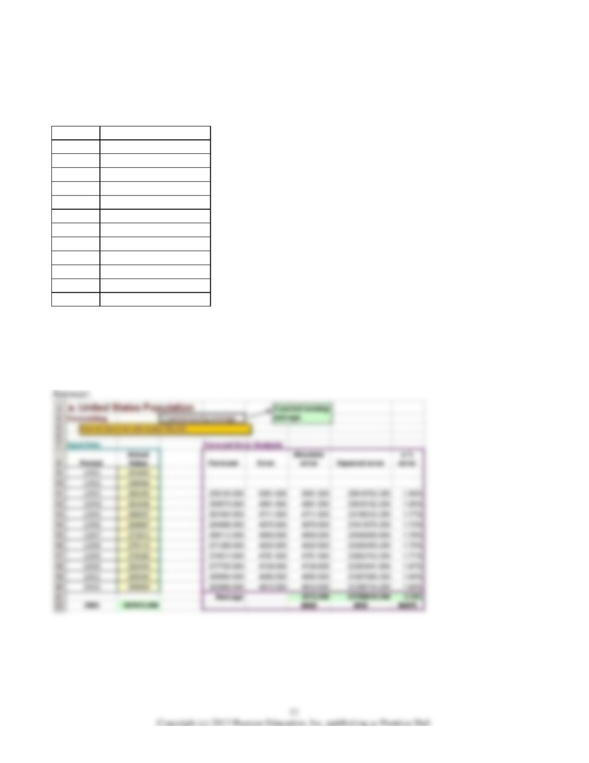
1) Refer to the table above.
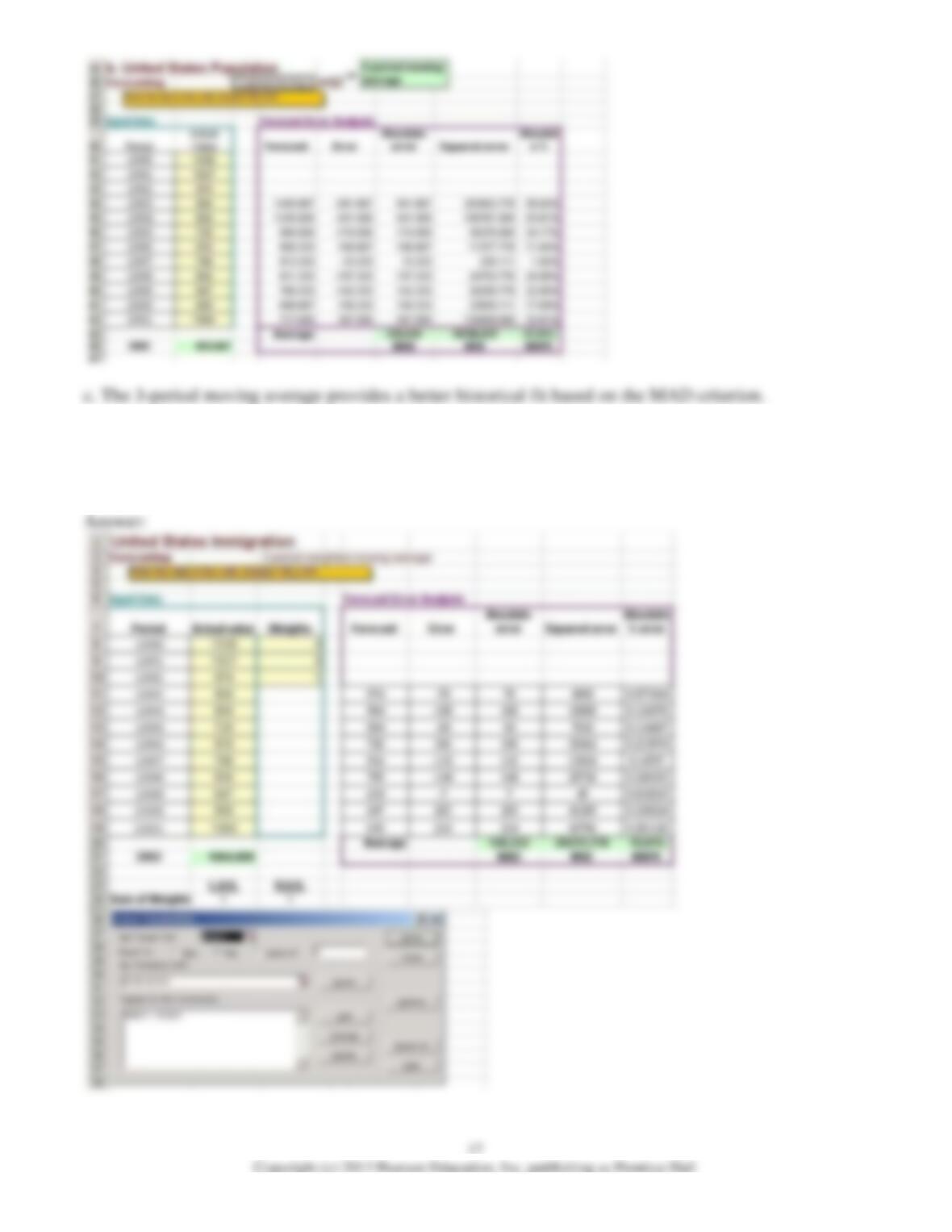
a. Use a 2-period moving average to forecast the population of the United States in 2003.
b. Use a 3-period moving average to forecast the population of the United States in 2003.
c. Which averaging period provides a better historical fit based on the MAD criterion?
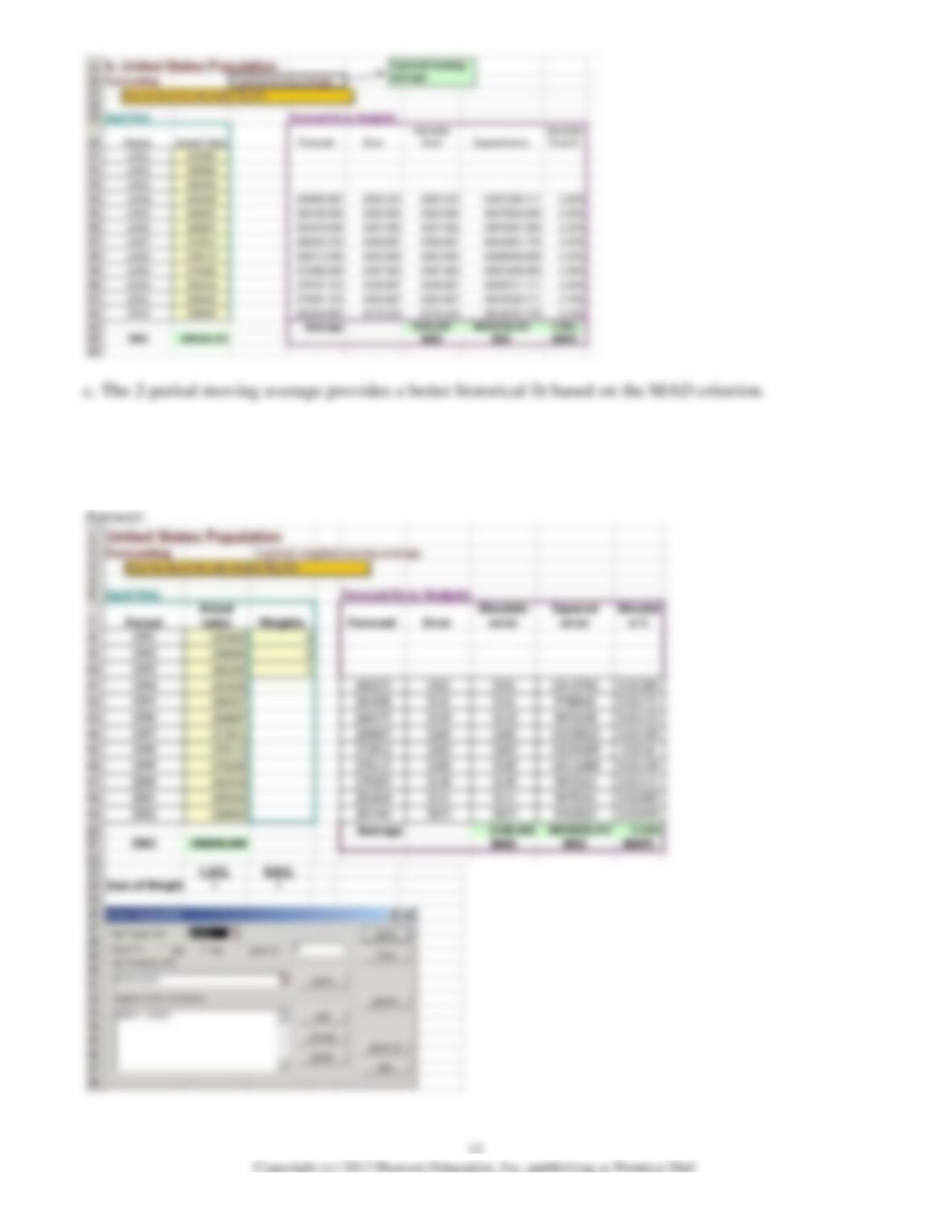
2) Refer to the table above. Use a 3-period weighted moving average to forecast the population of the
United States in 2003. Use Solver to determine the optimal weights based on minimizing the MAD
criterion.
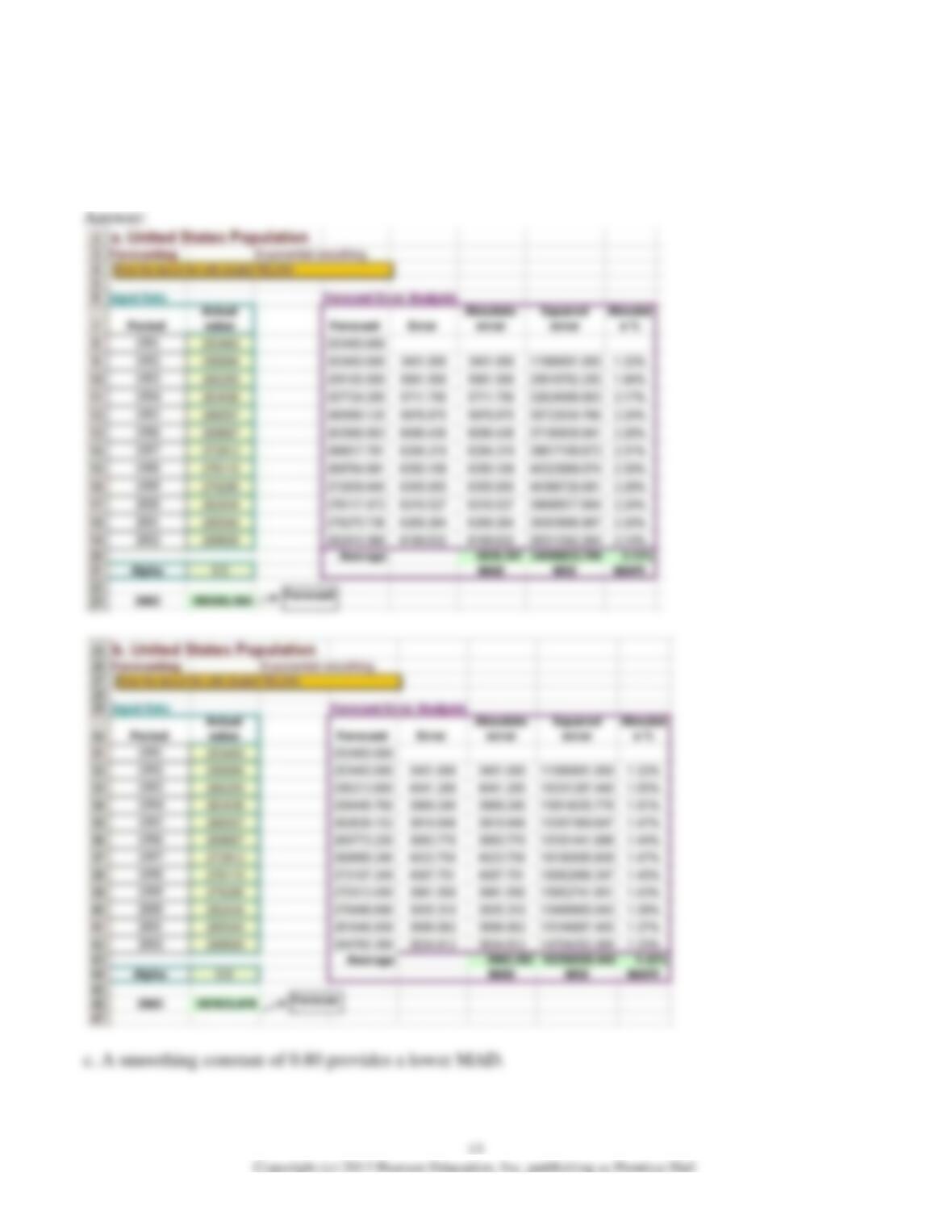
3) Refer to the table above.
a. Use exponential smoothing with a smoothing constant of 0.5 to forecast the population of the United
States in 2003.
b. Use exponential smoothing with a smoothing constant of 0.8 to forecast the population of the United
States in 2003.
c. Which of the two methods provides a more accurate forecast based on the MAD criterion?
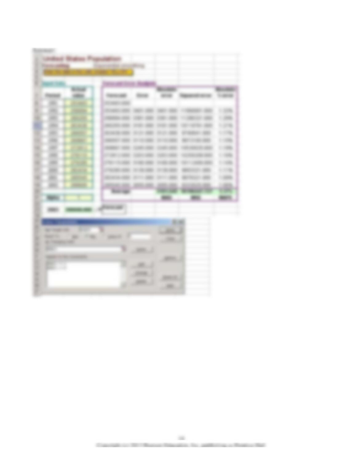
4) Refer to the table above. Using Solver to find the optimal alpha that minimizes MAD, use exponential
smoothing to forecast the population of the United States in 2003.
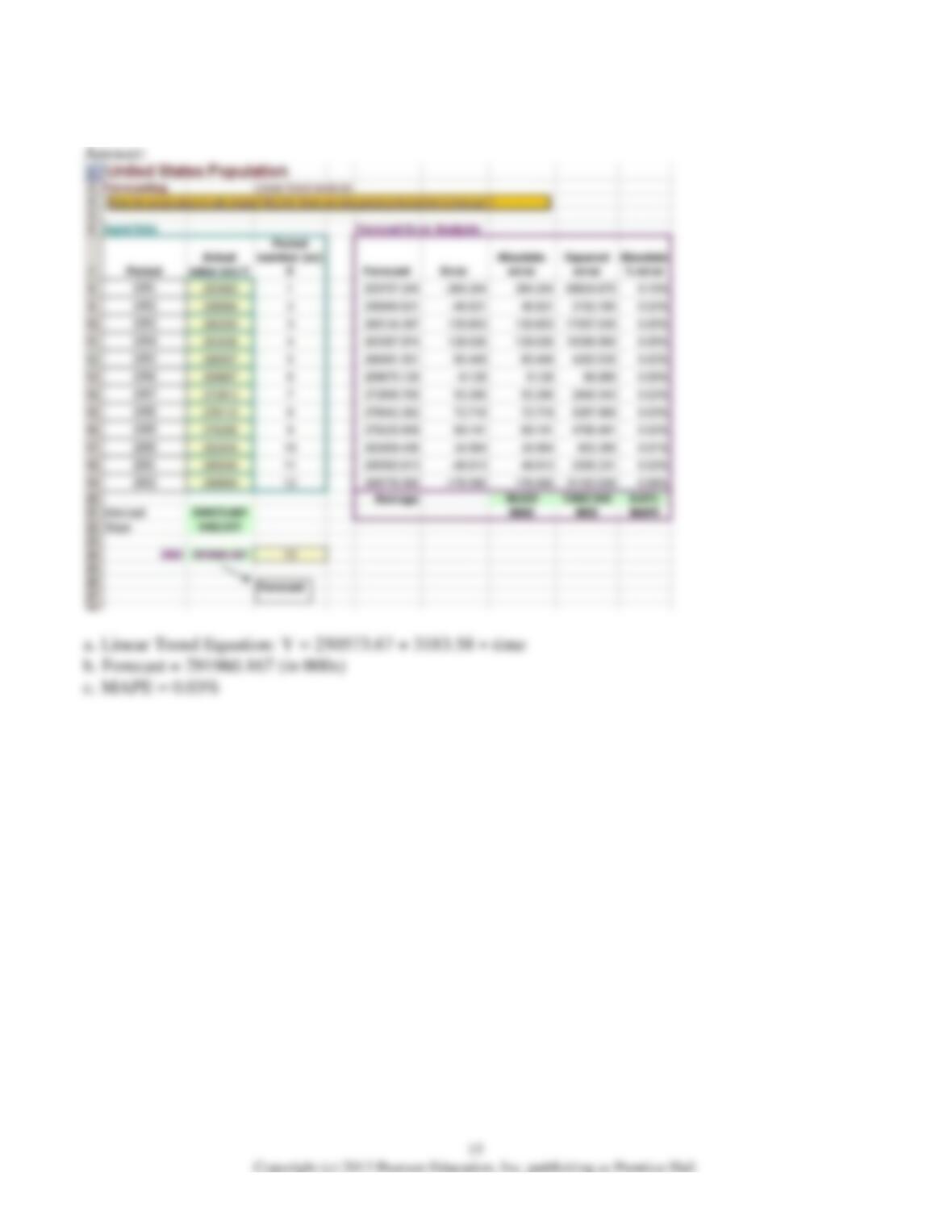
5) Refer to the table above. a. What is the linear trend equation that best fits the data?
b. What is the forecast of the population of the United States in 2003 using the linear trend equation?
c. What is the MAPE for this method?

Use this information to answer the following questions.
The following data, provided by the U.S. Bureau of Citizenship and Immigration Services, represent the
number of immigrants admitted to the United States, in thousands, from 1990-2001.
Year
No. of Immigrants
(in 000s)
1990
1536
1991
1827
1992
974
1993
904
1994
804
1995
720
1996
916
1997
798
1998
654
1999
647
2000
850
2001
1064
6) Refer to the table above.
a. Use a 2-period moving average to forecast the number of immigrants in 2002.
b. Use a 3-period moving average to forecast the number of immigrants in 2002.
c. Which averaging period provides a better historical fit based on the MAD criterion?
7) Refer to the table above. Use a 3-period weighted moving average to forecast the number of
immigrants in 2002. Use Solver to determine the optimal weights based on minimizing the MAD
criterion.
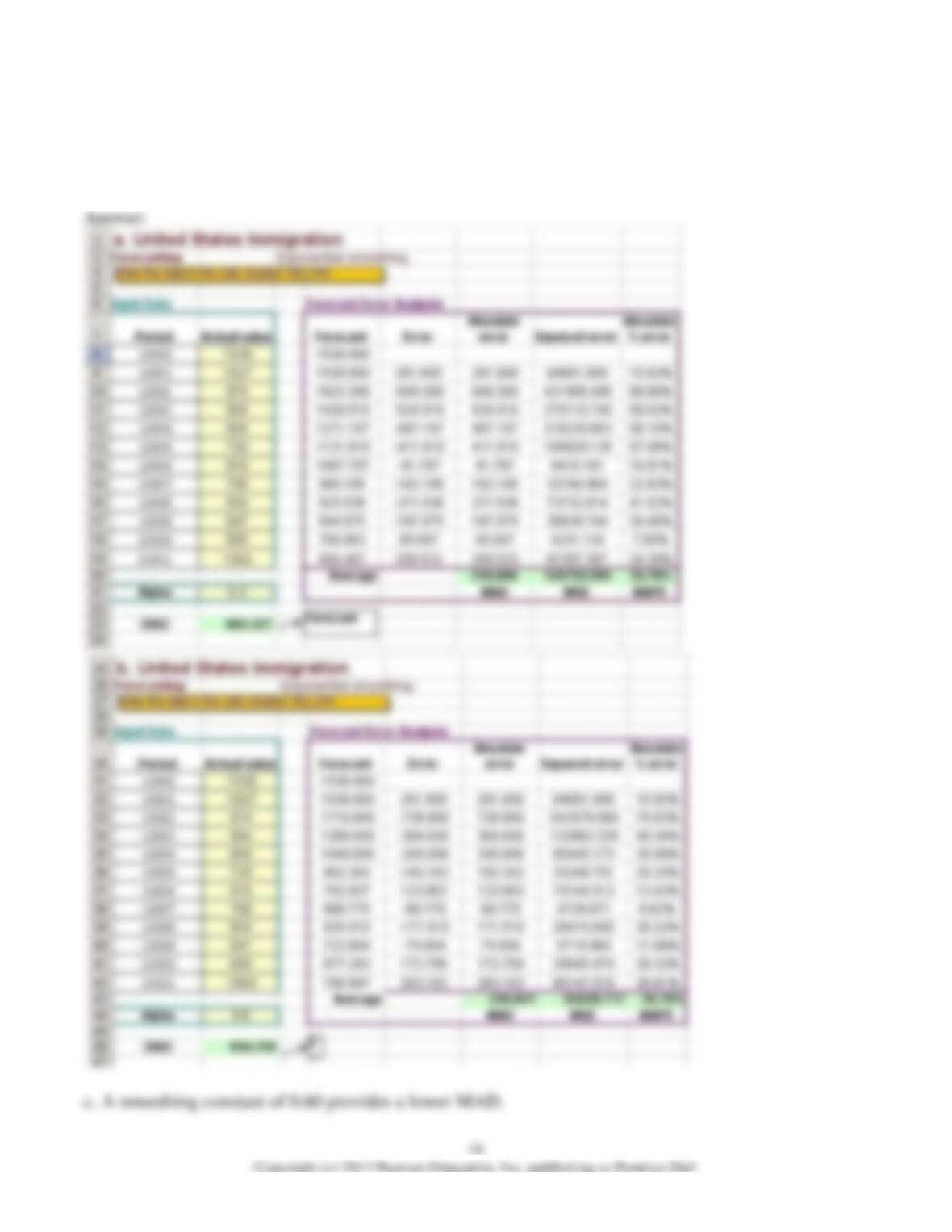
8) Refer to the table above.
a. Use exponential smoothing with a smoothing constant of 0.3 to forecast the number of immigrants in
2002.
b. Use exponential smoothing with a smoothing constant of 0.6 to forecast number of immigrants in
2002.
c. Which of the two methods provides a more accurate forecast based on the MAD criterion?
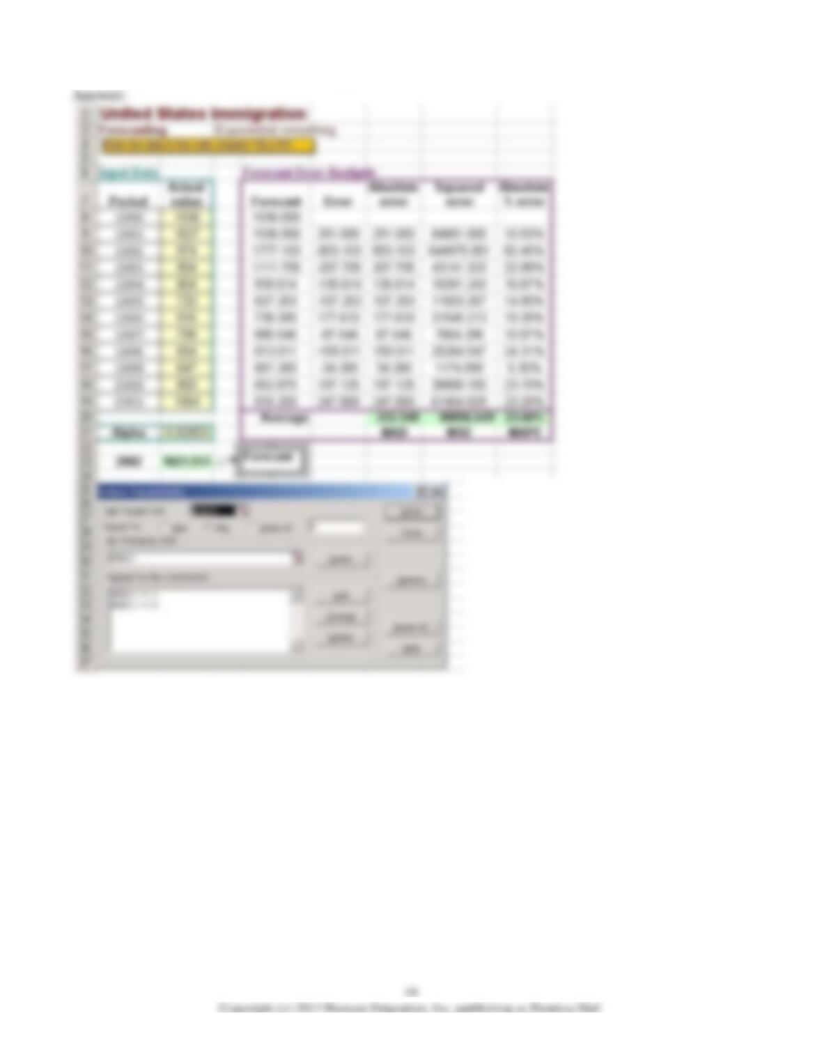
9) Refer to the table above. Using Solver to find the optimal alpha that minimizes MAD, use exponential
smoothing to forecast the number of immigrants in 2002.
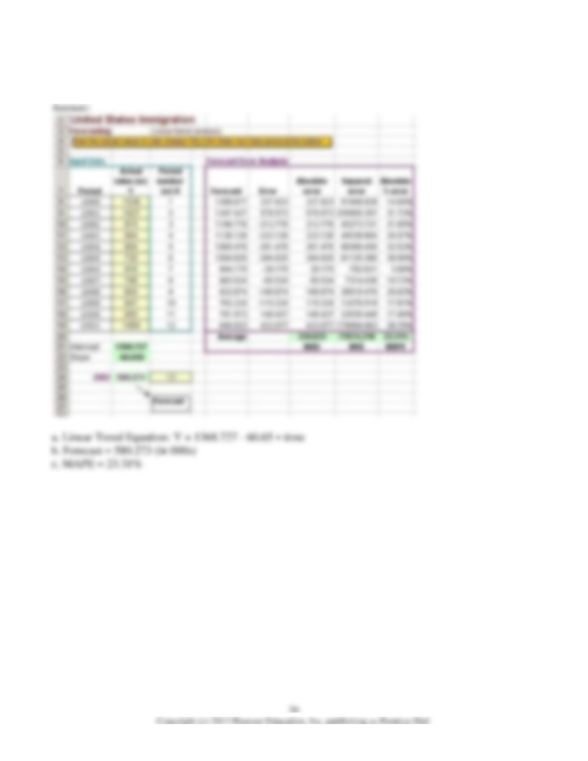
10) Refer to the table above.
a. What is the linear trend equation that best fits the data?
b. What is the forecast of the number of immigrants in 2002 using the linear trend equation?
c. What is the MAPE for this method?