Chapter 10 – Introduction to Simulation Modeling
1. The primary difference between simulation models and other types of spreadsheet models is that simulation models
contain ____:
a.
deterministic inputs
b.
random numbers
c.
output cells
d.
constraints
b
1
2. Which of the following is not one of the important distinctions of probability distributions?
a.
Discrete versus continuous
b.
Symmetric versus skewed
c.
Bounded versus unbounded
d.
Positive versus negative
d
1
3. Discrete distributions are sometimes used in place of continuous distributions:
a.
because they are more accurate
b.
because they are more simple
c.
when we don’t know the mean and variance of the distribution
d.
when we need to generate a histogram
b
1
4. The RAND() function in excel models which of the following probability distributions?
a.
Normal(0,1)
b.
Uniform(0,1)
c.
Normal(−1,1)
d.
Uniform(−1,1).
b
1
5. If x is a random number between 0 and 1, then we can use x to simulate a variable that is uniformly distributed between
100 and 200 using the formula:
a.
100 + x
b.
200 − x
c.
100 + 100x
d.
200x
c
1
6. A distribution for modeling the time it takes to serve a customer at a bank is probably:
a.
symmetric
b.
left skewed
Chapter 10 – Introduction to Simulation Modeling
c.
right skewed
d.
uniform
b
1
7. Which of the following statements is true regarding the Normal distribution?
a.
It is always the appropriate distribution in simulation modeling
b.
It does not permit negative values
c.
There is a 95% chance that values will be within ± 2 standard deviations of the mean
d.
All of these options
c
1
8. Which of the following statements is true regarding the Triangular distribution?
a.
It is a discrete distribution with a minimum, maximum and most likely value
b.
It is more flexible and intuitive than the normal distribution
c.
It is a symmetric distribution
d.
All of these options
b
1
9. When n is reasonably large and p isn’t too close to 0 or 1, the binomial distribution can be well approximated by which
of the following distributions?
a.
Uniform distribution
b.
Normal distribution
c.
Triangular distribution
d.
None of these options
b
1
10. If a model contains uncertain outputs, it can be very misleading to build a deterministic model by using the means of
the inputs to predict an output. This is called the:
a.
Law of Large Numbers.
b.
Flaw of Averages
c.
Law of Inevitable Disappointment
d.
Central Limit Theorem
b
1
11. One of the primary advantages of simulation models that they enable managers to answer what-if questions about
changes in systems without actually changing the systems themselves.
a.
True
b.
False
True
1
Chapter 10 – Introduction to Simulation Modeling
12. Excel’s standard functions, along with the RAND function, can be used to generate random numbers from many
different types of probability distributions.
a.
True
b.
False
True
1
13. The three parameters required to specify a triangular distribution are the minimum, mean and maximum.
a.
True
b.
False
False
1
14. A common guideline for constructing a 95% confidence interval is to place upper and lower bounds one standard error
on either side of the mean.
a.
True
b.
False
False
1
15. RISKSIMTABLE is an @RISK function for running several simulations simultaneously, one for each setting of an
input or decision variable.
a.
True
b.
False
True
1
16. When the value of a decision variable has been optimized by running several simulations, attitude toward risk should
no longer be relevant.
a.
True
b.
False
False
1
17. It is usually fairly straightforward to predict the shape of the output distribution from the shape(s) of the input
distribution(s).
a.
True
b.
False
False
1
18. A correlation matrix must always have 1’s along its diagonal (because a variable is always perfectly correlated with
itself) and numbers between −1 and +1 elsewhere.
a.
True
b.
False
True
Chapter 10 – Introduction to Simulation Modeling
19. A correlation matrix must always be symmetric, so that the correlations above the diagonal are a mirror image of those
below it.
a.
True
b.
False
True
1
20. Correlation between two random input variables may change the mean of an output, but it will not affect the
variability and shape of an output distribution.
a.
True
b.
False
False
1
Exhibit 10-1
A company is in the planning phase of constructing a new production facility. It wants to build a simulation model for the
economics of the facility, and one key uncertain input is the construction cost. For each of the scenarios in the questions
below, choose an “appropriate” distribution, together with its parameters, and explain your choice.
21. Refer to Exhibit 10–1. Company management currently has no idea what the distribution of the construction cost is.
All they can state is that “we think it will be somewhere between $5,000,000 and $8,000,000.”
The “no idea” suggests the uniform distribution, with a lower bound of $5M and an upper bound of $8M.
1
22. Refer to Exhibit 10–1. A little later on, management still believes the upper and lower bounds for the costs are $5M
and $8M, but now they can also state that “we believe the most likely value is about $6.5M.”
This suggests a triangular distribution, with a min of $5M, most likely value of $6.5M, and max of $8M.
1
23. Refer to Exhibit 10–1. Management believes the facility construction time will be somewhere from 5 to 9 months.
They believe the probabilities of the extremes (5 and 9 months) are both 10%, and the probabilities will vary linearly from
those endpoints to a most likely value at 7 months.
This is a general discrete distribution. We just have to choose the probabilities of the values 5 to 9 so that they
increase and then decrease linearly, and add up to 1: P(5)=0.1, P(6)=0.225, P(7)=0.35, P(8)=0.225, P(9)=0.1.
1
24. Refer to Exhibit 10–1. Engineering also believes the construction time will be from 5 to 9 months. However, they
believe that 7 months is twice as likely as either 6 months or 8 months and that either of these latter possibilities is three
times as likely as either 5 months or 9 months.
This is another general discrete distribution, where we have to choose the probabilities so that they have the
specified ratios, and add up to 1: P(5)=0.072, P(6)=0.215, P(7)=0.43, P(8)=0.215, P(9)=0.072.
1
25. If you add n lognormally distributed random numbers, the mean of the distribution for the sum is the sum of the
individual means, and the variance of the distribution of the sum is the individual variances. This result is difficult to
prove mathematically, but it is easy to demonstrate with simulation. To do so, run a simulation where you add three
1
Chapter 10 – Introduction to Simulation Modeling
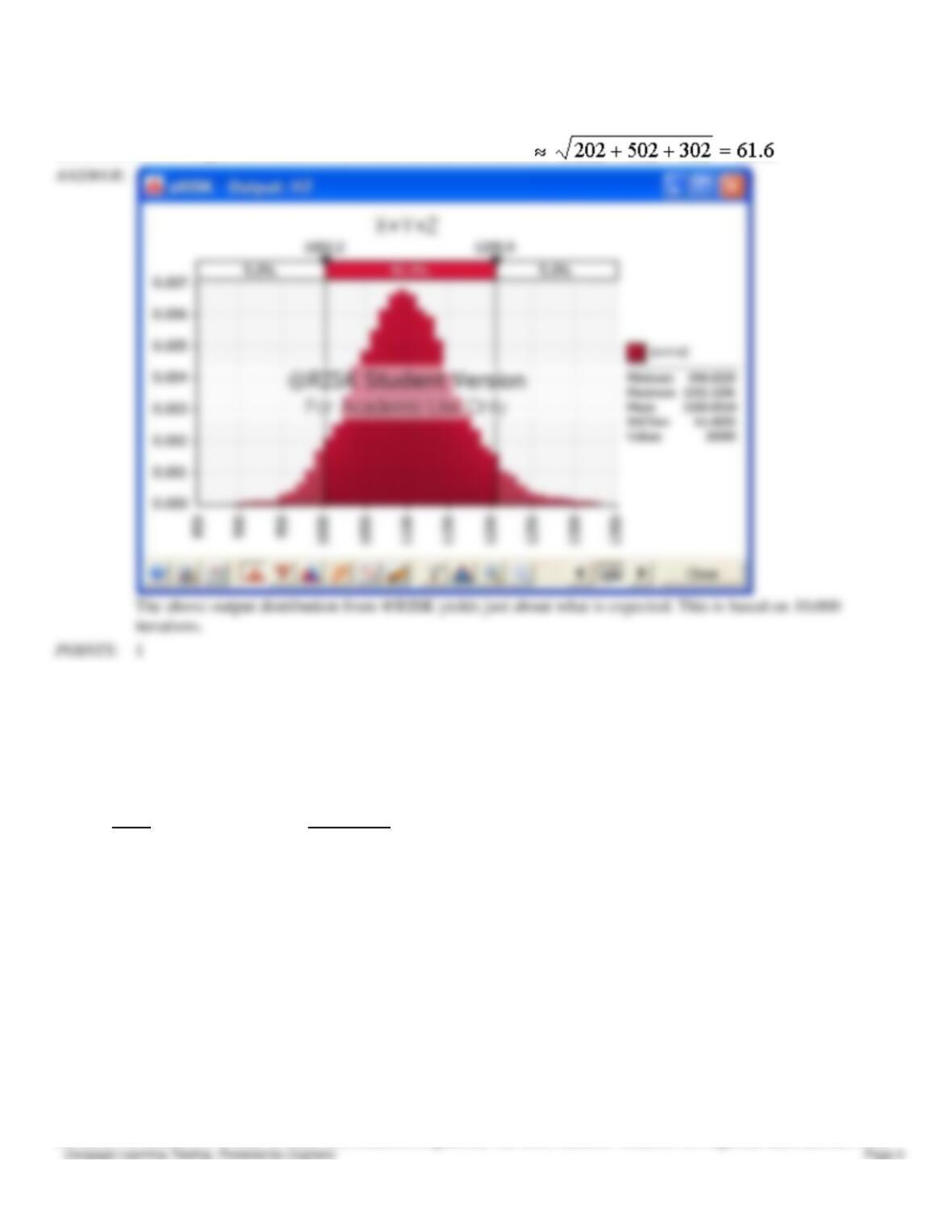
lognormally distributed random numbers, with means of 300, 700 and 100, and standard deviations of 20, 50, and 30,
respectively. Your single output variable should be the sum of these three numbers. Verify with @RISK that the
distribution of this output has a mean of 1,000 and standard deviation .
iterations.
1
Exhibit 10-2
A large apparel company wants to determine the profitability of one of its most popular products, a particular type of
jacket. Demand is uncertain, due to economic conditions, competition, weather and other factors, and the following
probability distributions have been estimated for each of the company’s three regions:
Estimate of Sales in Region 1
Units
Probability
9,000
0.05
10,000
0.10
11,000
0.15
12,000
0.35
13,000
0.25
14,000
0.10
Estimate of Sales in Region 2
Smallest Value:
5000 units
Most Likely Value:
7000 units
Largest Value:
12000 units
Estimate of Sales in Region 3
Minimum Value:
6000 units
Maximum Value:
9000 units
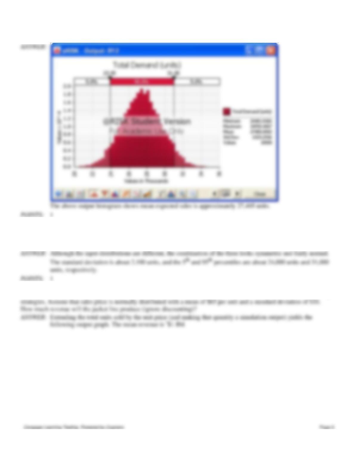
26. Refer to Exhibit 10–2. Use @RISK distributions to generate the three random variables for regional sales and derive a
Chapter 10 – Introduction to Simulation Modeling
distribution for the total sales. What is the expected total sales?
27. Refer to Exhibit 10–2. Total sales is a product of three different types of input distributions. What does the output
distribution look like? What is the standard deviation of the total sales? What are the 5th and 95th percentiles of this
distribution?
28. Refer to Exhibit 10–2. Suppose the jacket sales price also varies, depending on the individual retailers and their pricing
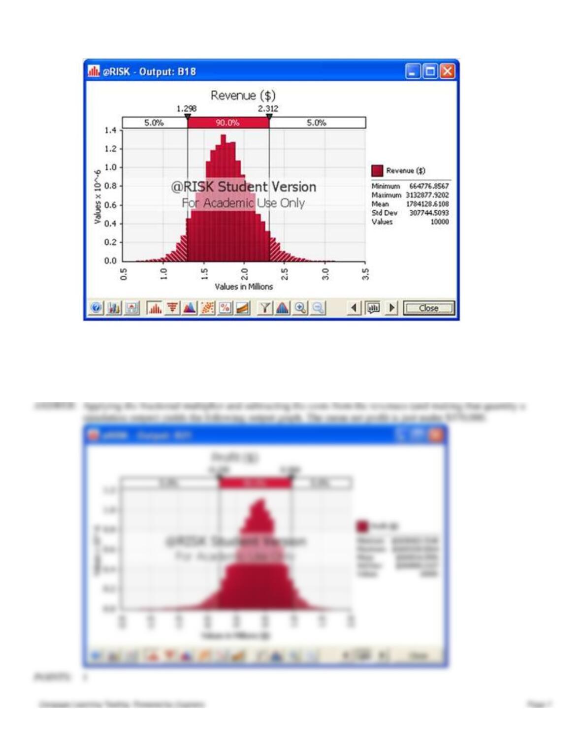
Chapter 10 – Introduction to Simulation Modeling
POINTS:
1
29. Refer to Exhibit 10–2. Finally, suppose the apparel company receives an uncertain fraction of the total retail revenue
from its retailers, modeled as a Triangular(0.70,0.75,0.80) distribution, and then must subtract production and operations
costs, which are modeled as a Lognormal distribution with mean of $1,000,000 and standard deviation of $300,000. In
that case, what is the expected net profit from the jacket line?
POINTS:
1
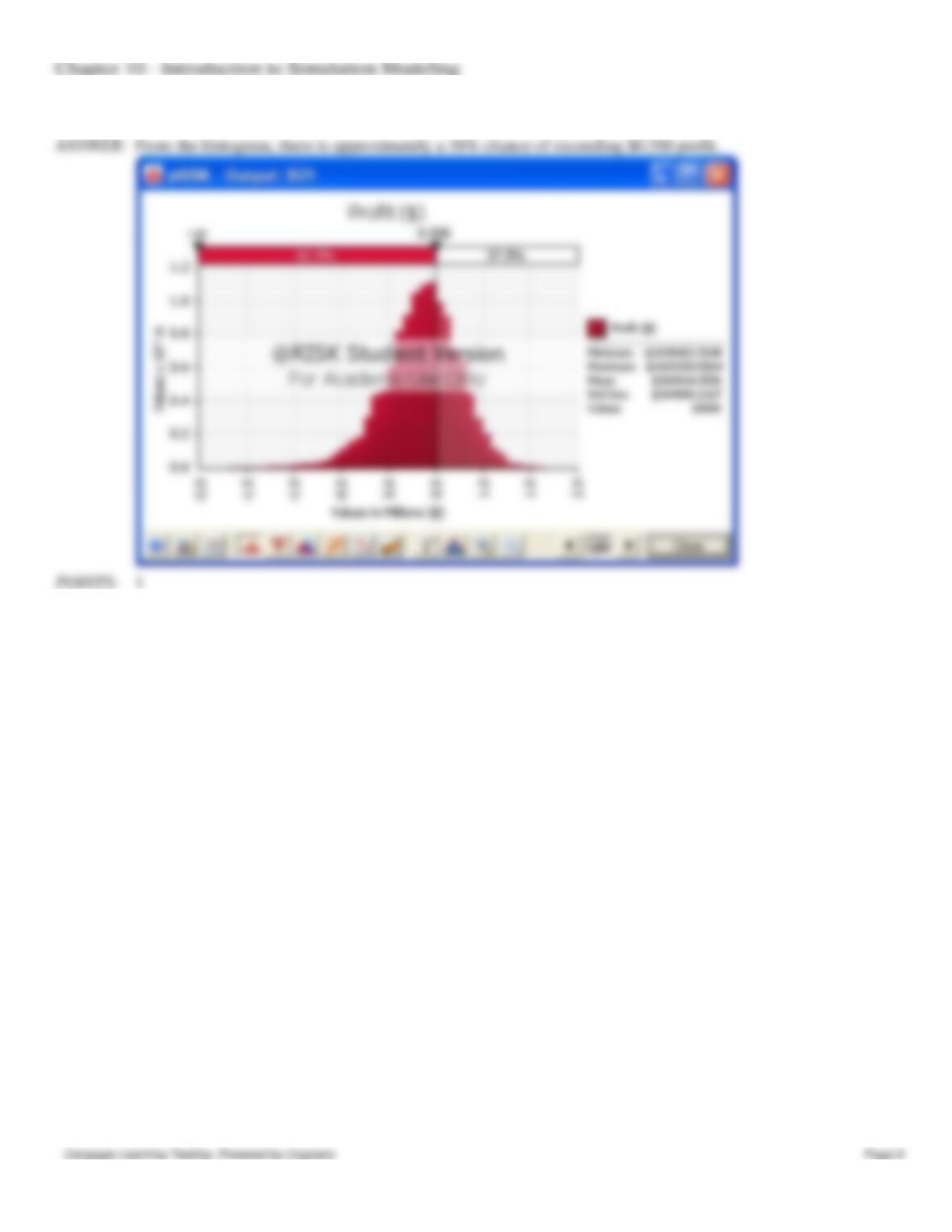
30. Refer to Exhibit 10–2. What is the probability that the apparel company will exceed a profit at least $0.5M from the
jacket line?