Cost Accounting: A Managerial Emphasis, 6e
Chapter 10 – Quantitative Analyses of Cost Functions
11) The new cost analyst in your accounting department has just received a computer-generated report
that contains the results of a simple regression program for cost estimation. The summary results of the
report appear as follows:
Variable Coefficient Standard Error t-Value
Constant $35.92 $16.02 2.24
Predictor variable $563.80 $205.40 2.74
r2 = 0.75
Required:
a. What is the cost estimation equation according to the report?
b. What is the goodness of fit? What does it tell about the estimating equation?
10.4 Explain ways to clean up dirty data.
1) The ideal database for estimating cost functions quantitatively includes values for the predictor
variable over a wide range.
2) For cost estimation purposes data must be collected using both time-series data and cross-sectional
data.

Cost Accounting: A Managerial Emphasis, 6e
Chapter 10 – Quantitative Analyses of Cost Functions
3) Which of the following is TRUE concerning the collection of data to be used in estimating a cost
function?
A) Data should contain observations for periods both before and after a major economic or technological
change.
B) The time periods used to measure the outcome variable and the cost driver(s) should not be
concurrent.
C) Both time series data and cross-sectional data are relevant, although both are not required.
D) All data should be viewed as being representative of the normal relationship between the outcome
variable and the cost driver.
E) Data should contain observations for periods both before and after a major economic or technological
change, and, both time series data and cross-sectional data are required.
4) Data collection problems arise when
A) data are recorded electronically rather than manually.
B) accrual-basis costs are used rather than cash-basis costs.
C) outliers are removed.
D) purely inflationary price effects are removed.
E) fixed and variable costs are not separately identified and both are allocated to products on a per unit
basis.
5) A better database for estimating cost functions has the following characteristics:
A) Fixed costs are allocated as if they are variable costs.
B) Extreme observations are adjusted or removed.
C) Time periods differ for measuring items included in the dependent variable and the cost driver(s).
D) Homogeneous relationships between individual cost items in the outcome variable pool and cost
drivers may not be present.
E) There is no causal, economically plausible relationship between individual cost items in a
heterogeneous mixed pool and a single cost driver.
Cost Accounting: A Managerial Emphasis, 6e
Chapter 10 – Quantitative Analyses of Cost Functions
6) Cross-sectional data analysis includes
A) using a variety of time periods to measure the dependent variable.
B) using the highest and lowest observation.
C) analyzing different cost drivers.
D) comparing information in different cost pools.
E) observing different entities during the same time period.
7) Brad Henry has just purchased the film studio of a movie company that specializes in action
adventures. He found that the company did not try to estimate the cost of making a movie. Instead it just
gave the producer a budget and told him/her to make a movie within budget. Mr. Henry does not like the
former movie-budget concept and desires to establish a formal cost estimation system.
Required:
What are some of the potential problems that may be encountered in changing from a budget to a cost
estimation movie-making system?
Cost Accounting: A Managerial Emphasis, 6e
Chapter 10 – Quantitative Analyses of Cost Functions
8) The ideal database for estimating cost functions has two characteristics:
1. It contains at least 31 reliably measured observations of the predictor variable and the outcome
variable.
2. It includes values for the predictor variable over a wide range.
Unfortunately, management accountants rarely have the advantage of working with a database that has
both characteristics.
Required:
Following are a list of data problems that may be encountered. Select three, then for each selection
describe the describe the cause/effect of the problem and provide a remedy.
1. The time period for measuring the outcome variable does not match the period for measuring the
predictor variable.
2. Fixed costs are allocated as if they were variable.
3. Data are either unavailable for all observations or not uniformly available.
4. Extreme values of observations, or outliers, occur when recording costs.
5. There is no causal, economically plausible relationship between the individual cost items in a
heterogeneous mixed pool and a single cost driver.
6. Inflation affects the outcome variable, the predictor variable(s), or both.

Cost Accounting: A Managerial Emphasis, 6e
Chapter 10 – Quantitative Analyses of Cost Functions
10.5 Appendix. Use statistics reported from simple linear regression to reliably and
confidently predict the range within which the total value of the cost pool will fall. Use
multiple linear regression to determine how more than one cost driver (Xi) improves
the prediction of the MOH cost value (y).
1) Statistical significance is determined by comparing the t-Stat to a threshold call degrees of freedom.
2) Spurious correlation refers to a repetitive coincidence of input measures with little causality to the
outcome variable.
3) The standard error of the estimated coefficient indicates whether a relationship exists between the
predictor variable and the outcome variable that cannot be attributed to chance alone.
4) Multicollinearity exists in multiple linear regression when two or more predictor variables are highly
correlated with each other.
5) What criteria are available in determining which of two alternate cost function estimates is better for a
particular management decision?
A) goodness of fit
B) economic plausibility
C) the significance of the difference between the costs associated with the highest and lowest observations
of the cost driver
D) the significance of the difference between the unit values for the highest and lowest observations of the
cost driver
E) the goodness of fit and economic plausibility

Cost Accounting: A Managerial Emphasis, 6e
Chapter 10 – Quantitative Analyses of Cost Functions
6) Which of the following is/are one of the criteria used when a manager evaluates an estimated cost
function for decision making purposes?
A) economic plausibility
B) goodness of fit
C) irrelevant high-low outliers
D) specifications analysis
E) economic plausibility and goodness of fit
7) In multiple regression, when two or more independent variables are correlated with one another, the
situation is known as
A) heteroscedasticity.
B) homoscedasticity.
C) spurious correlation.
D) autocorrelation.
E) multicollinearity.
8) Multicollinearity exists when which of the following conditions is present?
A) At least two variables change due to changes in the cost driver.
B) There are at least two cost pools (usually separated for fixed and variable costs).
C) The underlying value of the coefficient can only be explained in relation to dependent variables.
D) There are two or more statistically significant observations of at least two independent variables.
E) Two or more independent variables are highly correlated with each other.
9) In regression analysis, the term independence of residuals means
A) the residual term for any one observation is not related to the residual term of any other observation.
B) the data exhibit serial correlation.
C) the data exhibit autocorrelation.
D) there is a systematic pattern of positive residuals.
E) there is a systematic pattern of either only positive or only negative residuals.
Cost Accounting: A Managerial Emphasis, 6e
Chapter 10 – Quantitative Analyses of Cost Functions
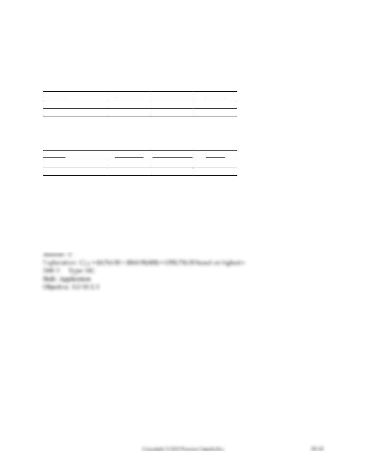
10) Larson’s Stables uses two different independent variables in two different equations to evaluate the
cost activities of training horses, trainer’s hours, and number of horses. The most recent year’s results of
the two regressions are as follows:
Trainer’s hours:
Variable
Coefficient
Standard Error
t-Value
Constant
913.32
198.12
4.61
Predictor Variable
20.90
2.94
7.11
r2 = 0.56
Number of horses:
Variable
Coefficient
Standard Error
t-Value
Constant
4,764.50
1,073.09
4.44
Predictor Variable
864.98
247.14
3.50
r2 = 0.63
What is the estimated cost for the coming year if 16,000 trainer hours are incurred and the stable has 400
horses to be trained based on the best cost driver?
A) $33,555.50
B) $99,929.09
C) $350,756.50
D) $335,313.32
E) $13,844,444.50
Cost Accounting: A Managerial Emphasis, 6e
Chapter 10 – Quantitative Analyses of Cost Functions
11) C. M. Chain was to manufacture 1,000 chain saws next month. Its accountant has provided the
following analysis of the total manufacturing costs.
Variable
Coefficient
Standard Error
t-Value
Constant
200
143.88
1.39
Predictor Variable
400
183.49
2.18
r2 = 0.71
What is the estimated cost of producing the 1,000 chain saws?
A) $400,200
B) $284,142
C) $200,400
D) $18,000
E) $9,000
12) Goodness-of-fit measures how well the predicted values in a cost estimating equation
A) match the cost driver.
B) match the actual cost observations.
C) fit the coefficient of determination.
D) rely on the independent variable.
E) rely on the dependent variable
13) Which of the following statements about a high correlation between two variables s and t is FALSE?
A) s may cause t.
B) t may cause s.
C) They both may be affected by a third variable.
D) The correlation establishes an economically plausible relationship between costs and their cost drivers.
E) The correlation may be due to random chance.
Cost Accounting: A Managerial Emphasis, 6e
Chapter 10 – Quantitative Analyses of Cost Functions
Use the information below to answer the following question(s).
Bernie Company used regression analysis to predict the annual cost of indirect materials. The results
were as follows:
Indirect Materials Cost Explained by Units Produced
Constant
$4,378
Standard error of Y estimate
$912
R – squared
0.9183
No. of observations
12
Degrees of freedom
10
X coefficient
2.35
Standard error of coefficient(s)
0.437525
14) The linear cost function is
A) Y =.$918 + 0.44X.
B) Y = $912 + $1.03X.
C) Y = $4,020 + $0.92X.
D) Y = $4,378+ $0.92X.
E) Y = $4,378 + $2.35X.
15) The coefficient of determination is
A) 22.00000.
B) 12.00000.
C) 2.350000.
D) 0.918300.
E) 0.437525.

Cost Accounting: A Managerial Emphasis, 6e
Chapter 10 – Quantitative Analyses of Cost Functions
16) Simple linear regression differs from multiple linear regression in that
A) multiple linear regression uses all available data to estimate the cost function whereas simple linear
regression only uses simple data.
B) simple linear regression is limited to the use of only the outcome variables and multiple linear
regression can use both outcome and predictor variables.
C) simple linear regression uses only one predictor variable and multiple linear regression uses more
than one predictor variable.
D) simple linear regression uses only one outcome variable and multiple linear regression uses more than
one outcome variable.
E) the lease squares technique cannot be used for simple linear regression whereas it can be used for
multiple linear regression.
17) A major concern that arises with multiple linear regression is multicollinearity, which exists
A) in simple linear regression, when the dependent variable is not normally distributed.
B) in simple linear regression, when the r2 statistic is low.
C) in multiple linear regression, when the r2 statistic is low.
D) in multiple linear regression, when two or more independent variables are correlated with one
another.
E) in multiple linear regression, when spurious correlation exists.
Cost Accounting: A Managerial Emphasis, 6e
Chapter 10 – Quantitative Analyses of Cost Functions
18) A Manufacturing Company uses two different independent variables in two different equations to
evaluate the cost activities of the packaging department, machine-hours and number of packages. The
most recent month’s results of the two regressions are as follows:
Machine hours:
Variable
Coefficient
Standard Error
t-Value
Constant
652.32
209.75
3.11
Predictor Variable
44.30
24.61
1.88
r2 = 0.29
Number of packages:
Variable
Coefficient
Standard Error
t-Value
Constant
65.08
75.04
2.20
Predictor Variable
4.30
2.00
2.15
r2 = 0.61
Required:
a. What are the estimating equations for each cost driver?
b. Which cost driver is best and why?
Cost Accounting: A Managerial Emphasis, 6e
Chapter 10 – Quantitative Analyses of Cost Functions
19) Newton Company used least squares regression analysis to obtain the following output:
Payroll Department Cost
Explained by Number of Employees
Constant $5,800
Standard error of Y estimate 630
r2 0.8924
Number of observations 20
X coefficient(s) $1.902
Standard error of coefficient(s) 0.0966
Required:
a. What is the total fixed cost?
b. What is the variable cost per employee?
c. Prepare the linear cost function.
d. What is the coefficient of determination? Comment on the goodness of fit.
Cost Accounting: A Managerial Emphasis, 6e
Chapter 10 – Quantitative Analyses of Cost Functions
20) Schotte Manufacturing Company uses two different independent variables (machine–hours and
number of packages) in two different equations to evaluate costs of the packaging department. The most
recent results of the two regressions are as follows:
Machine-hours:
Variable Coefficient Standard Error t-Value
Constant $748.30 $341.20 2.19
Predictor Variable $52.90 $35.20 1.50
r2 = 0.33
Number of packages:
Variable Coefficient Standard Error t-Value
Constant $242.90 $75.04 3.24
Predictor Variable $5.60 $2.00 2.80
r2 = 0.73
Required:
a. What are the estimating equations for each cost driver?
b. Which cost driver is best and why?