CHAPTER 10—COMPARISONS INVOLVING MEANS, EXPERIMENTAL
DESIGN, AND ANALYSIS OF VARIANCE
MULTIPLE CHOICE
1. In making three pairwise comparisons, what is the experiment-wise Type I error rate
ew if the
comparison-wise Type I error rate
is .10?
a.
.001
b.
.081
c.
.271
d.
.300
2. The test statistic F is the ratio
a.
MSE/MST
b.
MSTR/MSE
c.
SSTR/SSE
d.
SSTR/SST
3. In testing for the equality of k population means, the number of treatments is
a.
k
b.
k − 1
c.
nT
d.
nT − k
4. The within-treatments estimate of
2 is called the
a.
sum of squares due to error
b.
mean square due to error
c.
sum of squares due to treatments
d.
mean square due to treatments
5. If we are testing for the equality of 3 population means, we should use the
a.
test statistic t
b.
test statistics z
c.
test statistic
2
d.
test statistic F
6. The process of allocating the total sum of squares and degrees of freedom to the various components is
referred to as
a.
replicating
b.
partitioning
c.
randomizing
d.
blocking
7. The process of using the same or similar experimental units for all treatments in order to remove a
source of variation from the error term is called
a.
replicating
b.
partitioning
c.
randomizing
d.
blocking
8. In analysis of variance, the levels of the factor are called the
a.
dependent variables
b.
experimental units
c.
treatments
d.
observations
9. In analysis of variance, the independent variable of interest is called the
a.
response variable
b.
factor
c.
experimental unit
d.
design variable
10. In analysis of variance, the dependent variable is called the
a.
response variable
b.
factor
c.
experimental unit
d.
design variable
11. If we reject the hypothesis H0:
1 =
2 =
3, we can conclude that
a.
all three population means are similar
b.
all three population means are equal
c.
all three population means are different
d.
at least two population means are different
12. If we are interested in testing whether the mean of population 1 is significantly larger than the mean of
population 2, the
a.
null hypothesis should state
1 −
2 0
b.
null hypothesis should state
1 −
2 0
c.
alternative hypothesis should state
1 −
2 0
d.
alternative hypothesis should state
1 −
2 0
13. If we are interested in testing whether the mean of population 1 is significantly smaller than the mean
of population 2, the
a.
null hypothesis should state
1 −
2 0
b.
null hypothesis should state
1 −
2 0
c.
alternative hypothesis should state
1 −
2 0
d.
alternative hypothesis should state
1 −
2 0
14. When developing an interval estimate for the difference between two sample means, with sample sizes
of n1 and n2,
a.
n1 must be equal to n2
b.
n1 must be smaller than n2
c.
n1 must be larger than n2
d.
n1 and n2 can be of different sizes
15. To construct an interval estimate for the difference between the means of two populations when the
standard deviations of the two populations are unknown, we must use a t distribution with (let n1 be the
size of sample 1 and n2 the size of sample 2)
a.
(n1 + n2) degrees of freedom
b.
(n1 + n2 − 1) degrees of freedom
c.
(n1 + n2 − 2) degrees of freedom
d.
n1 − n2 + 2
16. When each data value in one sample is matched with a corresponding data value in another sample, the
samples are known as
a.
corresponding samples
b.
matched samples
c.
independent samples
d.
None of these alternatives is correct.
17. Independent simple random samples are taken to test the difference between the means of two
populations whose variances are not known. The sample sizes are n1 = 32 and n2 = 40. The correct
distribution to use is the
a.
binomial distribution
b.
t distribution with 72 degrees of freedom
c.
t distribution with 71 degrees of freedom
d.
t distribution with 70 degrees of freedom
18. Independent simple random samples are taken to test the difference between the means of two
populations whose standard deviations are not known. The sample sizes are n1 = 25 and n2 = 35. The
correct distribution to use is the
a.
Poisson distribution
b.
t distribution with 60 degrees of freedom
c.
t distribution with 59 degrees of freedom
d.
t distribution with 58 degrees of freedom
19. If two independent large samples are taken from two populations, the sampling distribution of the
difference between the two sample means
a.
can be approximated by a Poisson distribution
b.
will have a variance of one
c.
can be approximated by a normal distribution
d.
will have a mean of one
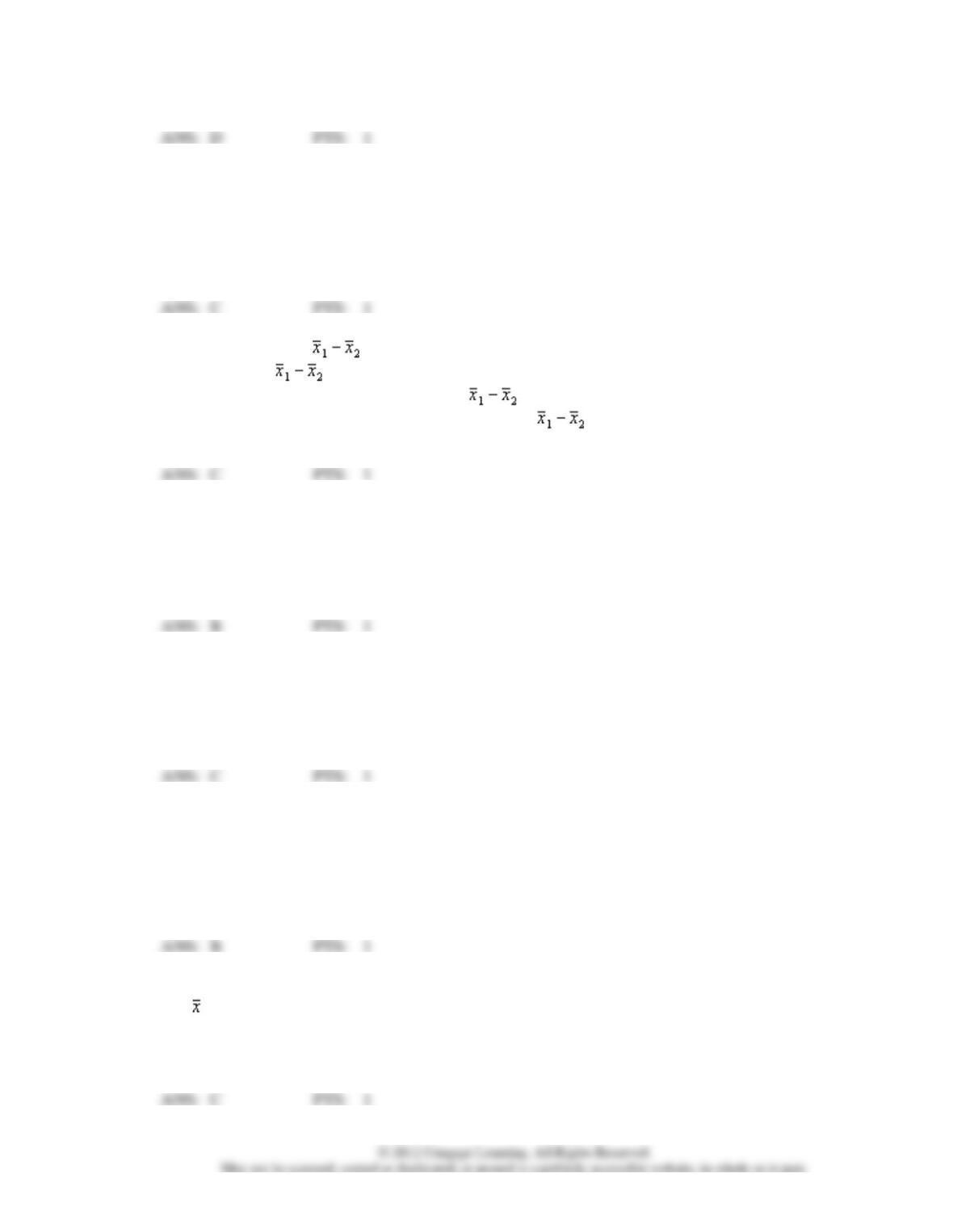
20. The standard error of is the
a.
variance of
b.
variance of the sampling distribution of
c.
standard deviation of the sampling distribution of
d.
difference between the two means
21. In an analysis of variance problem if SST = 120 and SSTR = 80, then SSE is
a.
200
b.
40
c.
80
d.
120
22. The required condition for using an ANOVA procedure on data from several populations is that the
a.
the selected samples are dependent on each other
b.
sampled populations are all uniform
c.
sampled populations have equal variances
d.
sampled populations have equal means
23. An ANOVA procedure is used for data that was obtained from four sample groups each comprised of
five observations. The degrees of freedom for the critical value of F are
a.
3 and 20
b.
3 and 16
c.
4 and 17
d.
3 and 19
24. In ANOVA, which of the following is not affected by whether or not the population means are equal?
a.
b.
between-samples estimate of 2
c.
within-samples estimate of 2
d.
None of these alternatives is correct.
25. A term that means the same as the term “variable” in an ANOVA procedure is
a.
factor
b.
treatment
c.
replication
d.
variance within
26. In order to determine whether or not the means of two populations are equal,
a.
a t test must be performed
b.
an analysis of variance must be performed
c.
either a t test or an analysis of variance can be performed
d.
a chi-square test must be performed
27. In a completely randomized design involving three treatments, the following information is provided:
Treatment 1
Treatment 2
Treatment 3
Sample Size
5
10
5
Sample Mean
4
8
9
The overall mean for all the treatments is
a.
7.00
b.
6.67
c.
7.25
d.
4.89
28. In a completely randomized design involving four treatments, the following information is provided.
Treatment 1
Treatment 2
Treatment 3
Treatment 4
Sample Size
50
18
15
17
Sample Mean
32
38
42
48
The overall mean (the grand mean) for all treatments is
a.
40.0
b.
37.3
c.
48.0
d.
37.0
29. An ANOVA procedure is used for data obtained from five populations. Five samples, each comprised
of 20 observations, were taken from the five populations. The numerator and denominator
(respectively) degrees of freedom for the critical value of F are
a.
5 and 20
b.
4 and 20
c.
4 and 99
d.
4 and 95
30. The critical F value with 8 numerator and 29 denominator degrees of freedom at = 0.01 is
a.
2.28
b.
3.20
c.
3.33
d.
3.64
31. An ANOVA procedure is used for data obtained from four populations. Four samples, each comprised
of 30 observations, were taken from the four populations. The numerator and denominator
(respectively) degrees of freedom for the critical value of F are
a.
3 and 30
b.
4 and 30
c.
3 and 119
d.
3 and 116
32. Which of the following is not a required assumption for the analysis of variance?
a.
The random variable of interest for each population has a normal probability distribution.
b.
The variance associated with the random variable must be the same for each population.
c.
At least 2 populations are under consideration.
d.
Populations have equal means.
33. In an analysis of variance, one estimate of 2 is based upon the differences between the treatment
means and the
a.
means of each sample
b.
overall sample mean
c.
sum of observations
d.
populations have equal means
Exhibit 10-1
Salary information regarding male and female employees of a large company is shown below.
Male
Female
Sample Size
64
36
Sample Mean Salary (in $1,000)
44
41
Population Variance
128
72
34. Refer to Exhibit 10-1. The point estimate of the difference between the means of the two populations
is
a.
-28
b.
3
c.
4
d.
4
35. Refer to Exhibit 10-1. The standard error for the difference between the two means is
a.
4
b.
7.46
c.
4.24
d.
2.0
36. Refer to Exhibit 10-1. At 95% confidence, the margin of error is
a.
1.96
b.
1.645
c.
3.920
d.
2.000
37. Refer to Exhibit 10-1. The 95% confidence interval for the difference between the means of the two
populations is
a.
0 to 6.92
b.
-2 to 2
c.
-1.96 to 1.96
d.
-0.92 to 6.92
38. Refer to Exhibit 10-1. If you are interested in testing whether or not the average salary of males is
significantly greater than that of females, the test statistic is
a.
2.0
b.
1.5
c.
1.96
d.
1.645
39. Refer to Exhibit 10-1. The p-value is
a.
0.0668
b.
0.0334
c.
1.336
d.
1.96
40. Refer to Exhibit 10-1. At 95% confidence, the conclusion is the
a.
average salary of males is significantly greater than females
b.
average salary of males is significantly lower than females
c.
salaries of males and females are equal
d.
None of these alternatives is correct.
Exhibit 10-2
The following information was obtained from matched samples.
The daily production rates for a sample of workers before and after a training program are shown
below.
Worker
Before
After
1
20
22
2
25
23
3
27
27
4
23
20
5
22
25
6
20
19
7
17
18
41. Refer to Exhibit 10-2. The point estimate for the difference between the means of the two populations
is
a.
-1
b.
-2
c.
0
d.
1
42. Refer to Exhibit 10-2. The null hypothesis to be tested is H0:
d = 0. The test statistic is
a.
-1.96
b.
1.96
c.
0
d.
1.645
43. Refer to Exhibit 10-2. The
a.
null hypothesis should be rejected
b.
null hypothesis should not be rejected
c.
alternative hypothesis should be accepted
d.
None of these alternatives is correct.
Exhibit 10-3
A statistics teacher wants to see if there is any difference in the abilities of students enrolled in
statistics today and those enrolled five years ago. A sample of final examination scores from students
enrolled today and from students enrolled five years ago was taken. You are given the following
information.
Today
Five Years Ago
82
88
2
112.5
54
n
45
36
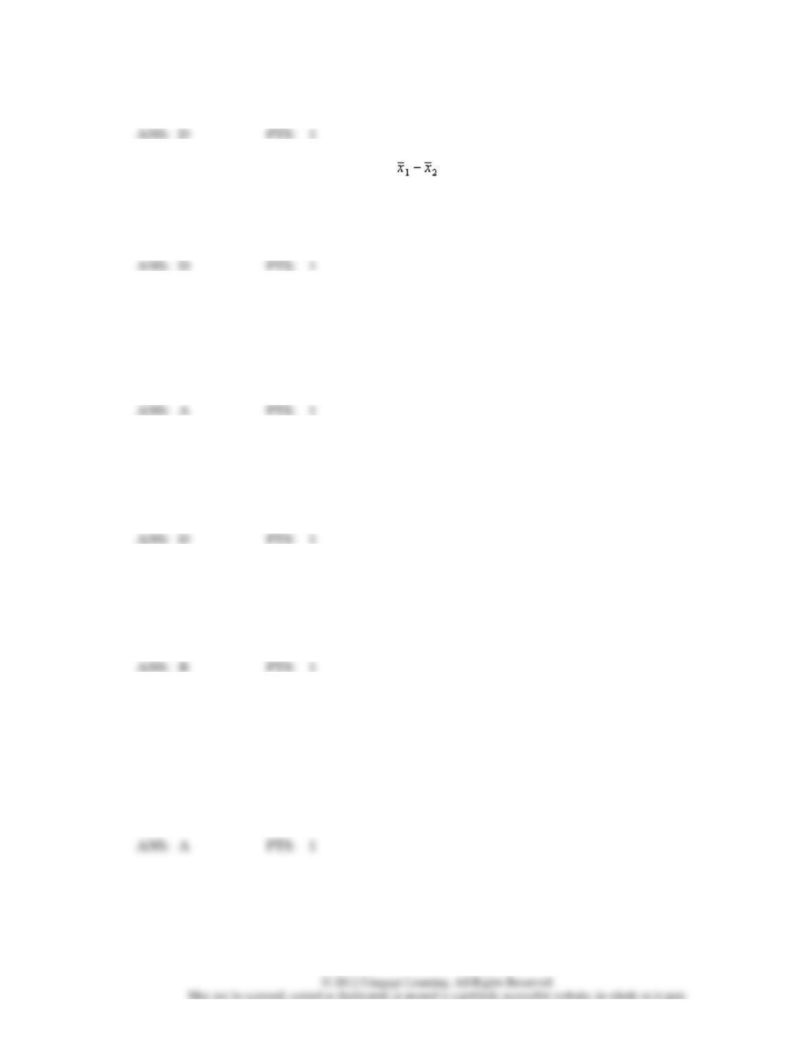
44. Refer to Exhibit 10-3. The point estimate for the difference between the means of the two populations
is
a.
58.5
b.
9
c.
-9
d.
-6
45. Refer to Exhibit 10-3. The standard error of is
a.
12.9
b.
9.3
c.
4
d.
2
46. Refer to Exhibit 10-3. The 95% confidence interval for the difference between the two population
means is
a.
-9.92 to -2.08
b.
-3.92 to 3.92
c.
-13.84 to 1.84
d.
-24.228 to 12.23
47. Refer to Exhibit 10-3. The test statistic for the difference between the two population means is
a.
-.47
b.
-.65
c.
-1.5
d.
-3
48. Refer to Exhibit 10-3. The p-value for the difference between the two population means is
a.
.0014
b.
.0027
c.
.4986
d.
.9972
49. Refer to Exhibit 10-3. What is the conclusion that can be reached about the difference in the average
final examination scores between the two classes? (Use a .05 level of significance.)
a.
There is a statistically significant difference in the average final examination scores
between the two classes.
b.
There is no statistically significant difference in the average final examination scores
between the two classes.
c.
It is impossible to make a decision on the basis of the information given.
d.
There is a difference, but it is not significant.
Exhibit 10-4
The following information was obtained from independent random samples.
Assume normally distributed populations with equal variances.
Sample 1
Sample 2
Sample Mean
45
42
Sample Variance
85
90
Sample Size
10
12
50. Refer to Exhibit 10-4. The point estimate for the difference between the means of the two populations
is
a.
0
b.
2
c.
3
d.
15
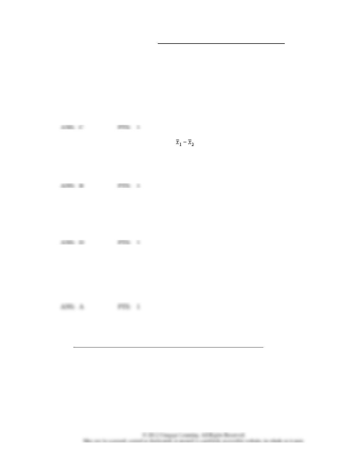
51. Refer to Exhibit 10-4. The standard error of is
a.
3.0
b.
4.0
c.
8.372
d.
19.48
52. Refer to Exhibit 10-4. The degrees of freedom for the t distribution are
a.
22
b.
21
c.
20
d.
19
53. Refer to Exhibit 10-4. The 95% confidence interval for the difference between the two population
means is
a.
-5.372 to 11.372
b.
-5 to 3
c.
-4.86 to 10.86
d.
-2.65 to 8.65
Exhibit 10-5
The following information was obtained from matched samples.
Individual
Method 1
Method 2
1
7
5
2
5
9
3
6
8
4
7
7
5
5
6
54. Refer to Exhibit 10-5. The point estimate for the difference between the means of the two populations
(method 1 − method 2) is
a.
-1
b.
0
c.
-4
d.
2
55. Refer to Exhibit 10-5. The 95% confidence interval for the difference between the two population
means is
a.
-3.776 to 1.776
b.
-2.776 to 2.776
c.
-1.776 to 2.776
d.
0 to 3.776
56. Refer to Exhibit 10-5. The null hypothesis tested is H0:
d = 0. The test statistic for the difference
between the two population means is
a.
2
b.
0
c.
-1
d.
-2
57. Refer to Exhibit 10-5. If the null hypothesis is tested at the 5% level, the null hypothesis
a.
should be rejected
b.
should not be rejected
c.
should be revised
d.
None of these alternatives is correct.
Exhibit 10-6
The management of a department store is interested in estimating the difference between the mean
credit purchases of customers using the store’s credit card versus those customers using a national
major credit card. You are given the following information.
Store’s Card
Major Credit Card
Sample size
64
49
Sample mean
$140
$125
Population standard deviation
$10
$8
58. Refer to Exhibit 10-6. A point estimate for the difference between the mean purchases of the users of
the two credit cards is
a.
2
b.
18
c.
265
d.
15
59. Refer to Exhibit 10-6. At 95% confidence, the margin of error is
a.
1.694
b.
3.32
c.
1.96
d.
15
60. Refer to Exhibit 10-6. A 95% confidence interval estimate for the difference between the average
purchases of the customers using the two different credit cards is
a.
49 to 64
b.
11.68 to 18.32
c.
125 to 140
d.
8 to 10
Exhibit 10-7
In order to estimate the difference between the average hourly wages of employees of two branches of
a department store, the following data have been gathered.
Downtown Store
North Mall Store
Sample size
25
20
Sample mean
$15
$14
Sample standard deviation
$2
$1
For this problem, the degrees of freedom are computed to be 36.
61. Refer to Exhibit 10-7. A point estimate for the difference between the two sample means is
a.
1
b.
2
c.
3
d.
4
62. Refer to Exhibit 10-7. A 95% interval estimate for the difference between the two population means is
a.
0.078 to 1.922
b.
1.922 to 2.078
c.
1.09 to 4.078
d.
1.078 to 2.922
Exhibit 10-8
In order to determine whether or not there is a significant difference between the hourly wages of two
companies, the following data have been accumulated.
Company A
Company B
Sample size
80
60
Sample mean
$16.75
$16.25
Population standard deviation
$1.00
$0.95
63. Refer to Exhibit 10-8. A point estimate for the difference between the two sample means is
a.
20
b.
0.50
c.
0.25
d.
1.00
64. Refer to Exhibit 10-8. The test statistic is
a.
0.098
b.
1.645
c.
2.75
d.
3.01
65. Refer to Exhibit 10-8. The p-value is
a.
0.0013
b.
0.0026
c.
0.0042
d.
0.0084
66. Refer to Exhibit 10-8. The null hypothesis
a.
should be rejected
b.
should not be rejected
c.
should be revised
d.
None of these alternatives is correct.
Exhibit 10-9
Two major automobile manufacturers have produced compact cars with the same size engines. We are
interested in determining whether or not there is a significant difference in the MPG (miles per gallon)
of the two brands of automobiles. A random sample of eight cars from each manufacturer is selected,
and eight drivers are selected to drive each automobile for a specified distance. The following data
show the results of the test.
Driver
Manufacturer A
Manufacturer B
1
32
28
2
27
22
3
26
27
4
26
24
5
25
24
6
29
25
7
31
28
8
25
27
67. Refer to Exhibit 10-9. The mean for the differences is
a.
0.50
b.
1.5
c.
2.0
d.
2.5
68. Refer to Exhibit 10-9. The test statistic is
a.
1.645
b.
1.96
c.
2.096
d.
2.256
69. Refer to Exhibit 10-9. At 90% confidence the null hypothesis
a.
should not be rejected
b.
should be rejected
c.
should be revised
d.
None of these alternatives is correct.
Exhibit 10-10
A local department store is studying the shopping habits of its customers. They think that the longer
customers spend in the store the more they buy. Their study resulted in the following information
regarding the amount of time women and men spent in a store.
Women
Men
Mean
6 minutes 12 seconds
5 minutes 46 seconds
Population Standard deviation
4 seconds
5 seconds
Sample size
32
50
70. Refer to Exhibit 10-10. The point estimate for the difference between the means of the two populations
is
a.
1 minute 26 seconds
b.
34 seconds
c.
26 seconds
d.
13 seconds
71. Refer to Exhibit 10-10. The point estimate for the standard deviation of the difference between the
means of the two populations is
a.
9
b.
-1
c.
-9
d.
1
72. Refer to Exhibit 10-10. The 95% confidence interval for the difference between the two population
means is
a.
24.04 to 27.96
b.
1.96
c.
-1.96 to 1.96
d.
-24.04 to 27.96
73. Refer to Exhibit 10-10. The test statistic for the difference between the two population means is
a.
1.96
b.
27.96
c.
21.00
d.
26.00
74. Refer to Exhibit 10-10. At 95% confidence, what is the conclusion for this study?
a.
There is a significant difference in the time spent in the store between men and women.
b.
There is no significant difference in the time spent in the store between men and women.
c.
It is impossible to make a decision on the basis of the information given.
d.
The sample sizes must be equal in order to answer this question.
Exhibit 10-11
To test whether or not there is a difference between treatments A, B, and C, a sample of 12
observations has been randomly assigned to the 3 treatments. You are given the results below.
Treatment
Observation
A
20
30
25
33
B
22
26
20
28
C
40
30
28
22
75. Refer to Exhibit 10-11. The null hypothesis for this ANOVA problem is
a.
1=
2
b.
1=
2=
3
c.
1=
2=
3=
4
d.
1=
2= … =
12
76. Refer to Exhibit 10-11. The mean square between treatments (MSTR) equals
a.
1.872
b.
5.86
c.
34
d.
36
77. Refer to Exhibit 10-11. The mean square within treatments (MSE) equals
a.
1.872
b.
5.86
c.
34
d.
36
78. Refer to Exhibit 10-11. The test statistic to test the null hypothesis equals
a.
0.944
b.
1.059
c.
3.13
d.
19.231
79. Refer to Exhibit 10-11. The null hypothesis is to be tested at the 1% level of significance. The p-value
is
a.
greater than 0.1
b.
between 0.1 and 0.05
c.
between 0.05 and 0.025
d.
between 0.025 and 0.01
80. Refer to Exhibit 10-11. The null hypothesis
a.
should be rejected
b.
should not be rejected
c.
should be revised
d.
None of these alternatives is correct.
Exhibit 10-12
In a completely randomized experimental design involving five treatments, 13 observations were
recorded for each of the five treatments (a total of 65 observations). The following information is
provided.
SSTR = 200 (Sum Square Between Treatments)
SST = 800 (Total Sum Square)
81. Refer to Exhibit 10-12. The sum of squares within treatments (SSE) is
a.
1,000
b.
600
c.
200
d.
1,600
82. Refer to Exhibit 10-12. The number of degrees of freedom corresponding to between treatments is
a.
60
b.
59
c.
5
d.
4
83. Refer to Exhibit 10-12. The number of degrees of freedom corresponding to within treatments is
a.
60
b.
59
c.
5
d.
4
84. Refer to Exhibit 10-12. The mean square between treatments (MSTR) is
a.
3.34
b.
10.00
c.
50.00
d.
12.00
85. Refer to Exhibit 10-12. The mean square within treatments (MSE) is
a.
50
b.
10
c.
200
d.
600
86. Refer to Exhibit 10-12. The test statistic is
a.
0.2
b.
5.0
c.
3.75
d.
15
87. Refer to Exhibit 10-12. If at 95% confidence we want to determine whether or not the means of the
five populations are equal, the p-value is
a.
between 0.05 and 0.10
b.
between 0.025 and 0.05
c.
between 0.01 and 0.025
d.
less than 0.01
Exhibit 10-13
Part of an ANOVA table is shown below.
ANOVA
Source of Variation
DF
SS
MS
F
Between Treatments
3
180
Within Treatments (Error)
Total
18
480
88. Refer to Exhibit 10-13. The mean square between treatments (MSTR) is
a.
20
b.
60
c.
300
d.
15
89. Refer to Exhibit 10-13. The mean square within treatments (MSE) is
a.
60
b.
15
c.
300
d.
20
90. Refer to Exhibit 10-13. The test statistic is
a.
2.25
b.
6
c.
2.67
d.
3
91. Refer to Exhibit 10-13. If at 95% confidence, we want to determine whether or not the means of the
populations are equal, the p-value is
a.
between 0.01 and 0.025
b.
between 0.025 and 0.05
c.
between 0.05 and 0.1
d.
greater than 0.1
Exhibit 10-14
Part of an ANOVA table is shown below.
ANOVA
Source of Variation
DF
SS
MS
F
Between Treatments
64
8
Within Treatments (Error)
2
Total
100
92. Refer to Exhibit 10-14. The number of degrees of freedom corresponding to between treatments is
a.
18
b.
2
c.
4
d.
3
93. Refer to Exhibit 10-14. The number of degrees of freedom corresponding to within treatments is
a.
22
b.
4
c.
5
d.
18
94. Refer to Exhibit 10-14. The mean square between treatments (MSTR) is
a.
36
b.
16
c.
64
d.
15
95. Refer to Exhibit 10-14. If at 95% confidence we want to determine whether or not the means of the
populations are equal, the p-value is
a.
greater than 0.1
b.
between 0.05 and 0.1
c.
between 0.025 and 0.05
d.
less than 0.01
96. Refer to Exhibit 10-14. The conclusion of the test is that the means
a.
are equal
b.
may be equal
c.
are not equal
d.
None of these alternatives is correct.
Exhibit 10-15
The following is part of an ANOVA table that was obtained from data regarding three treatments and a
total of 15 observations.
Source of Variation
DF
SS
Between Treatments
64
Error (Within Treatments)
96
97. Refer to Exhibit 10-15. The number of degrees of freedom corresponding to between treatments is
a.
12
b.
2
c.
3
d.
4
98. Refer to Exhibit 10-15. The number of degrees of freedom corresponding to within treatments is
a.
12
b.
2
c.
3
d.
15
99. Refer to Exhibit 10-15. The mean square between treatments (MSTR) is
a.
36
b.
16
c.
8
d.
32
100. Refer to Exhibit 10-15. The computed test statistics is
a.
32
b.
8
c.
0.667
d.
4
101. Refer to Exhibit 10-15. If at 95% confidence, we want to determine whether or not the means of the
populations are equal, the p-value is
a.
between 0.01 and 0.025
b.
between 0.025 and 0.05
c.
between 0.05 and 0.1
d.
greater than 0.1
102. Refer to Exhibit 10-15. The conclusion of the test is that the means
a.
are equal
b.
may be equal
c.
are not equal
d.
None of these alternatives is correct.
Exhibit 10-16
SSTR = 6,750
H0:
1 =
2 =
3 =
4
SSE = 8,000
Ha: at least one mean is different
nT = 20
103. Refer to Exhibit 10-16. The mean square between treatments (MSTR) equals
a.
400
b.
500
c.
1,687.5
d.
2,250
104. Refer to Exhibit 10-16. The mean square within treatments (MSE) equals
a.
400
b.
500
c.
1,687.5
d.
2,250
105. Refer to Exhibit 10-16. The test statistic to test the null hypothesis equals
a.
0.22
b.
0.84
c.
4.22
d.
4.5