Actual p-value = 0.0004
Since the p-value is < = 0.05, reject H0 (critical F = 2.17).
68. MNM, Inc. has three stores located in three different areas. Random samples of the daily sales of the
three stores (in $1,000) are shown below.
Store 1
Store 2
Store 3
9
10
6
8
11
7
7
10
8
8
13
11
At 95% confidence, test to see if there is a significant difference in the average sales of the three
stores. Show the complete ANOVA table.
ANOVA
Between Groups
Within Groups
Total
69. Ten observations were selected from each of 3 populations, and an analysis of variance was performed
on the data. The following are the results.
ANOVA
Source of Variation
SS
df
MS
F
Between Groups
82
?
?
?
Within Groups
162
?
?
Total
?
?
At 95% confidence, test to see if there is a significant difference among the means of the three
populations.
Source of Variation
Between Groups
Within Groups
6
Total
70. The following are the results from a completely randomized design consisting of 3 treatments.
ANOVA
Source of Variation
SS
df
MS
F
Between Groups
390
?
?
?
Within Groups
?
?
?
Total
558
23
Using = .05, test to see if there is a significant difference among the means of the three populations.
ANOVA
Source of Variation
Between Groups
Within Groups
8
Total
71. Eight observations were selected from each of 3 populations (total of 24 observations), and an analysis
of variance was performed on the data. The following are part of the results.
ANOVA
Source of Variation
SS
df
MS
F
Between Groups
216
?
?
?
Within Groups
252
?
?
Total
?
?
Using = .05, test to see if there is a significant difference among the means of the three populations.
Between Groups
Within Groups
Total
72. Random samples of individuals from three different cities were asked how much time they spend per
day watching television. The results (in minutes) for the three groups are shown below.
City I
City II
City III
260
182
211
280
190
190
240
220
247
260
240
300
a.
Compute the overall sample mean .
b.
At = 0.05, test to see if there is a significant difference in the averages of the three groups.
Show the complete ANOVA table.
235
b.
Between Groups
Within Groups
Total
Using the F table (2 numerator and 9 denominator degrees of freedom) for F = 7.19, the p–
value is between 0.01 and 0.025.
Actual p-value = 0.0136
Since the p-value is = 0.05, reject H0 (critical F = 4.26).
73. Three different brands of tires were compared for wear characteristics. From each brand of tire, ten
tires were randomly selected and subjected to standard wear-testing procedures. The average mileage
obtained for each brand of tire and sample variances (both in 1,000 miles) are shown below.
Brand A
Brand B
Brand C
Average Mileage
37
38
33
Sample variance
3
4
2
At 95% confidence, test to see if there is a significant difference in the average mileage of the three
brands.
Between Groups
Within Groups
Total
74. MOA, Inc. has three stores located in three different areas. Random samples of the sales of the three
stores (In $1,000) are shown below.
Store 1
Store 2
Store 3
46
34
33
47
36
31
45
35
35
42
39
45
a.
Compute the overall sample mean .
b.
At 95% confidence, test to see if there is a significant difference in the average sales of the
three stores. Show the complete ANOVA table.
39
b.
Between Groups
Within Groups
4
Total
Actual p-value = 0.0000
Since the p-value is = 0.05, reject H0 (critical F = 4.26).
75. In a completely randomized experimental design, 11 experimental units were used for each of the 4
treatments. Part of the ANOVA table is shown below.
ANOVA
Source of Variation
SS
df
MS
F
Between Groups
1500
?
?
?
Within Groups
?
?
?
Total
5500
?
a.
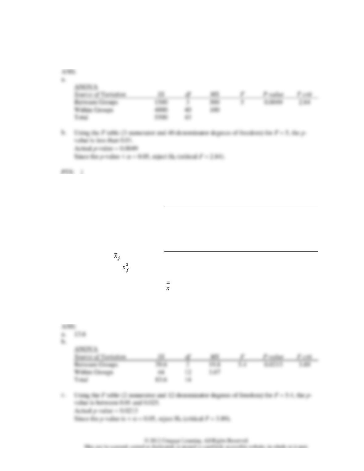
Determine all the missing values in the above table and fill in the blanks.
b.
Use = 0.05 to determine if there is any significant difference among the means of the four
treatments.
a.
Between Groups
Within Groups
Total
b.
Using the F table (3 numerator and 40 denominator degrees of freedom) for F = 5, the p–
Actual p-value = 0.0049
Since the p-value < = 0.05, reject H0 (critical F = 2.84).
76. Samples were selected from three populations. The data obtained are shown below.
Sample 1
Sample 2
Sample 3
10
16
15
9
14
15
12
13
16
13
14
14
16
10
17
Sample Mean ( )
11
15
14
Sample Variance ( )
3.33
2.4
5.5
a.
Compute the overall sample mean .
b.
Set up an ANOVA table for this problem.
c.
At 95% confidence test to determine whether there is a significant difference in the means of
the three populations.
a.
13.6
b.
Between Groups
Within Groups
Total
Using the F table (2 numerator and 12 denominator degrees of freedom) for F = 5.4, the p–
value is between 0.01 and 0.025.
Actual p-value = 0.0213
Since the p-value is < = 0.05, reject H0 (critical F = 3.89).
77. In a completely randomized experimental design, 16 experimental units were used for each of the 4
levels of the factor (i.e., 4 treatments). Part of the ANOVA table is shown below.
ANOVA
Source of Variation
SS
df
MS
F
Between Groups
?
?
100
?
Within Groups
?
?
?
Total
1560
?
a.
Determine all the missing values in the above table and fill in the blanks.
b.
Use = 0.05 to determine if there is any significant difference among the means of the four
groups.
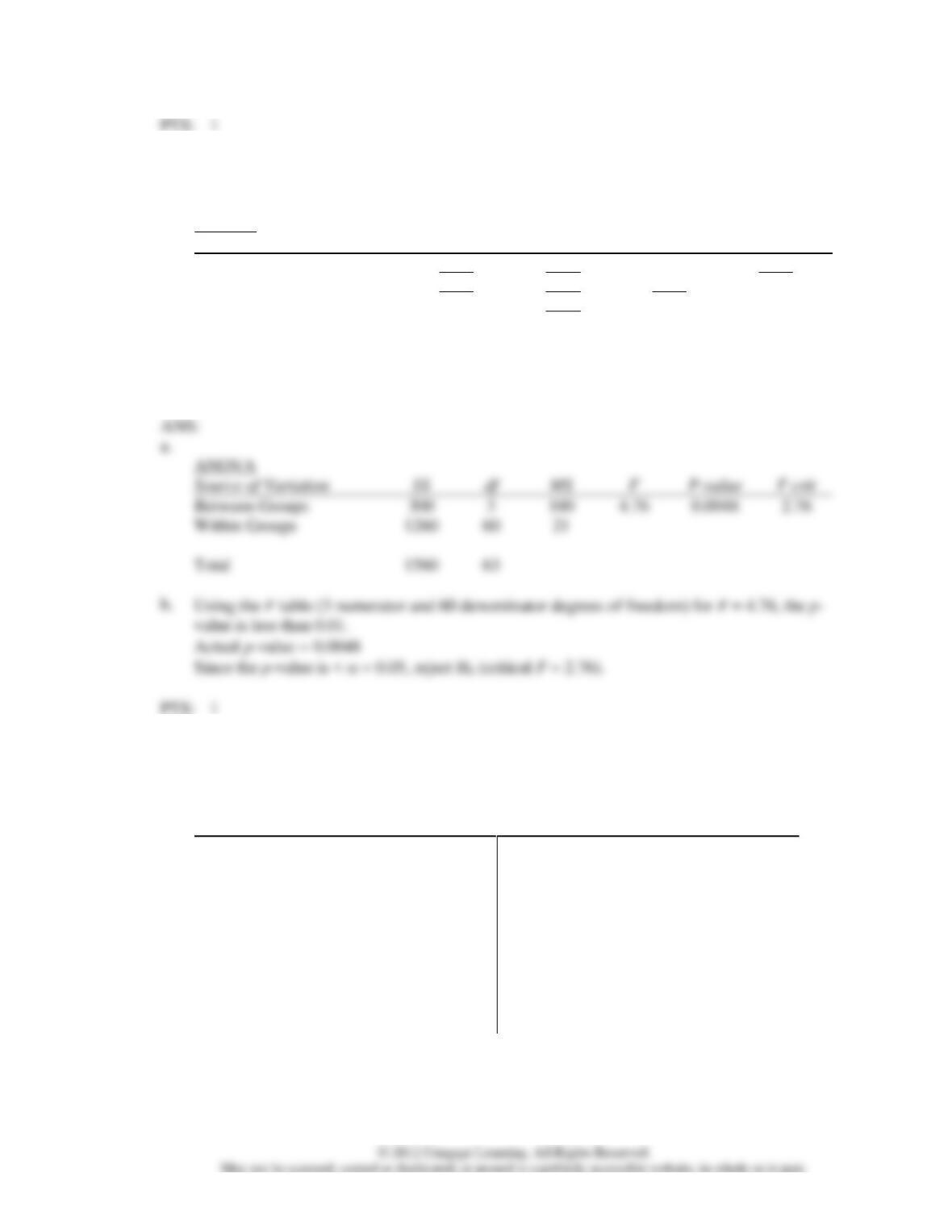
ANOVA
Source of Variation
Between Groups
Within Groups
Total
value is less than 0.01.
Actual p-value = 0.0048
Since the p-value is < = 0.05, reject H0 (critical F = 2.76).
78. Independent random samples of Company W employees were taken to compare salaries between
college graduates and high school graduates. Samples of size 30 were taken for each group. The results
follow.
Salary HS ($1000)
Salary College ($1000)
24.1
22.9
24.0
32.4
33.1
26.2
21.2
19.9
23.9
30.9
29.6
28.7
25.7
19.5
29.0
39.2
32.1
31.8
28.8
22.1
24.7
29.6
30.4
28.5
28.6
22.7
24.4
35.5
30.4
32.7
30.2
18.6
23.5
32.0
31.3
28.6
18.4
23.3
30.9
32.0
33.3
33.5
24.3
23.8
27.6
28.3
37.5
41.4
28.3
25.4
32.1
30.8
35.4
28.4
21.7
23.9
23.0
31.2
37.0
27.2
Use Excel to estimate the difference in average salaries between the two groups with a 95% level of
confidence.
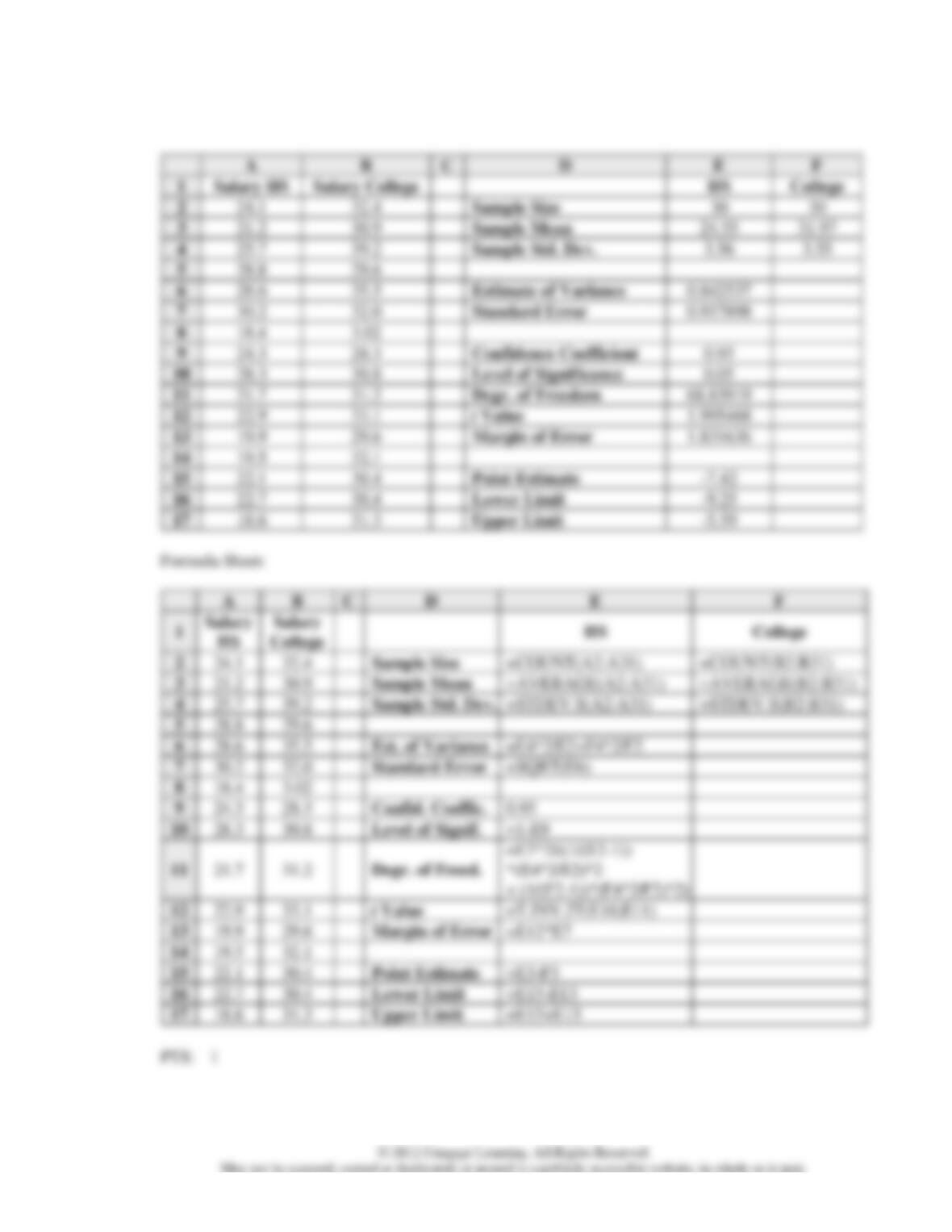
ANS:
Value Sheet
79. At a particular airport in the United States, independent samples of domestic flights from two airlines
were taken and the amount of time each flight was delayed was measured. The results follow.
Minutes Delayed
Minutes Delayed
Airline A
Airline B
0.0
33.7
0.0
7.2
25.6
31.8
0.0
34.6
38.9
36.2
0.0
41.6
27.3
24.7
34.8
43.1
44.5
0.0
38.9
39.4
41.8
41.5
42.1
7.8
35.3
23.5
39.5
12.8
34.5
38.1
35.7
33.0
29.0
32.9
41.3
31.8
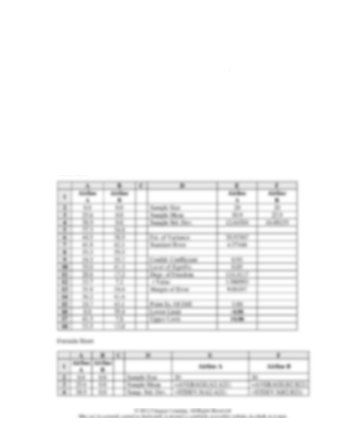
Use Excel to estimate the difference in average delay time between the two airlines with a 95% level
of confidence.
ANS:
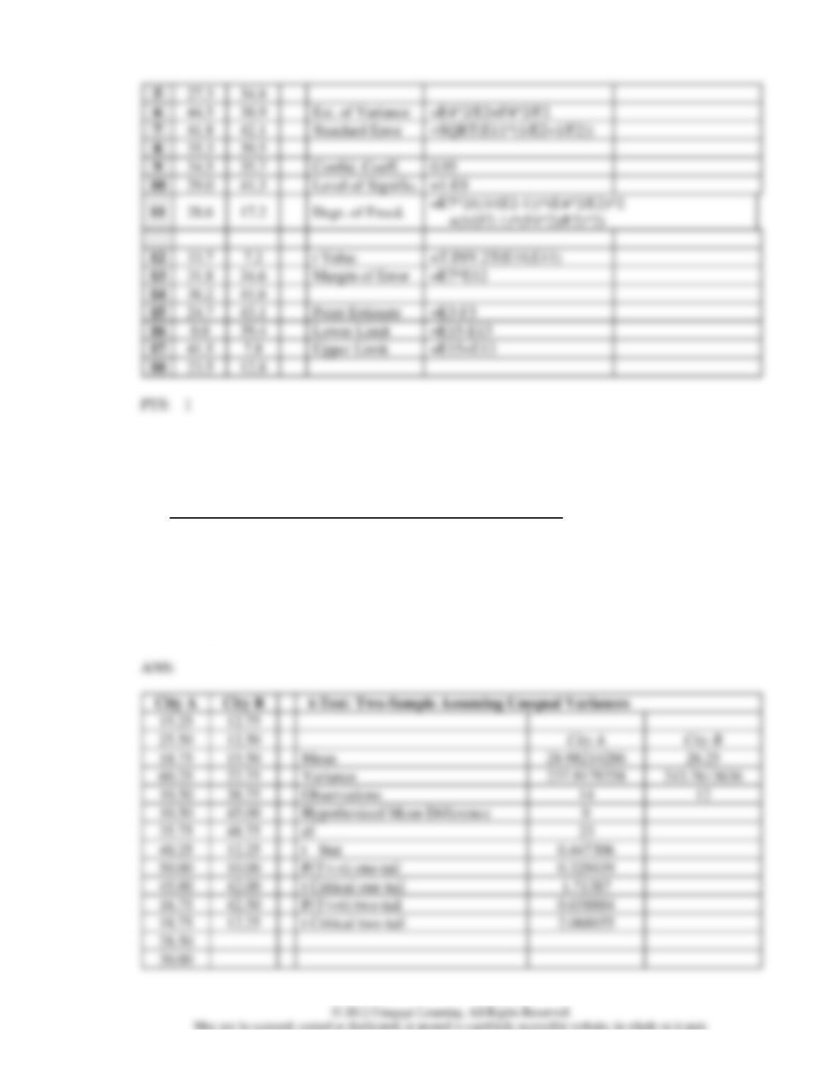
Value Sheet:
Sample Size
Sample Mean
30.9
25.9
Sample Std. Dev.
Est. of Variance
Standard Error
Confid. Coefficient
0.95
Level of Signific.
0.05
Degr. of Freedom
Margin of Error
Point Es. Of Diff.
5.00
Lower Limit
Upper Limit
Sample Size
20
20
Samp. Std. Dev.
=STDEV.S(A2:A21)
=STDEV.S(B2:B21)
80. Independent samples of commuters are taken from two cities. The following data represents the time
(in minutes) to drive to work. Use Excel to determine whether the average commuting times are
significantly different between the two cities. Use = .05.
City A
City B
15.25
40.25
12.75
48.75
25.50
50.00
12.50
12.25
18.75
45.00
15.50
10.00
60.25
16.75
22.75
42.00
10.50
18.75
38.75
42.50
10.50
28.50
45.00
12.25
35.75
30.00
0.329419
2.068655
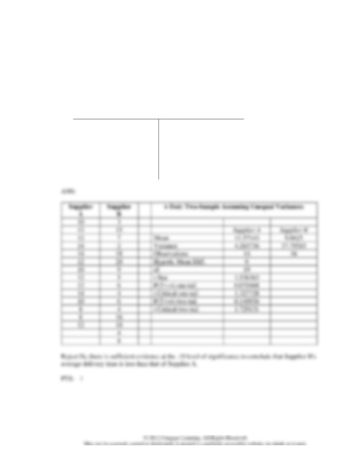
Do not reject H0; there is not sufficient evidence at the .05 level of significance to conclude that there
is a difference in mean commuting time between the two cities.
PTS: 1
81. The following independent samples show the delivery times for two suppliers of raw materials (in
days). A company currently uses Supplier A but will switch to Supplier B if its average delivery time
is less than that for Supplier A. Use Excel to conduct the appropriate hypothesis test. Use = .10.
Supplier A
Supplier B
10
12
3
6
13
13
15
4
12
14
7
6
14
10
2
4
14
8
18
16
12
8
20
18
10
12
9
4
5
8
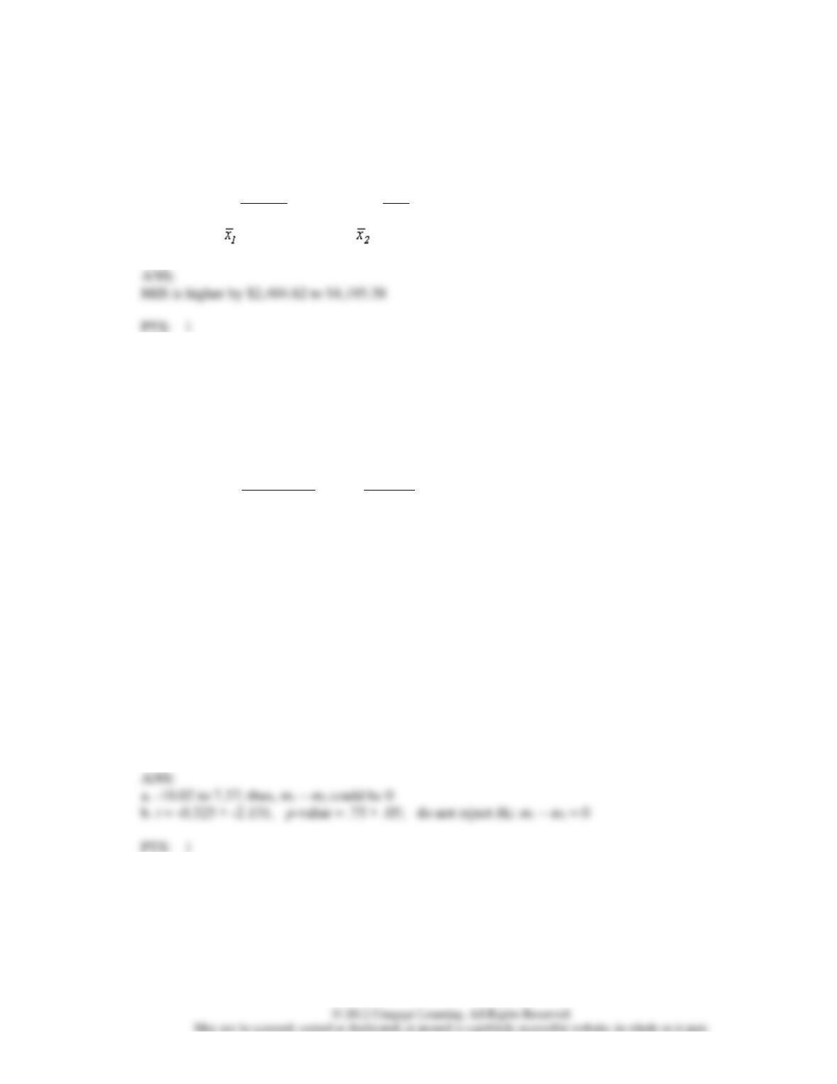
Mean
Variance
Observations
Hypoth. Mean Diff.
df
t Stat
P(T<=t) one-tail
t Critical one-tail
P(T<=t) two-tail
t Critical two-tail
82. Starting annual salaries for business school graduates majoring in finance and management
information systems (MIS) were collected in two independent random samples. Based on previous
studies, the population standard deviations for Finance and MIS salaries are estimated to be $2,100 and
$2,600, respectively. Use the following data to develop a 95% confidence interval estimate of the
difference between the starting salaries for the two majors.
Finance
MIS
n1 = 60
n2 = 50
= $43,200
= $46,500
83. A manager is thinking of providing, on a regular basis, in-house training for employees preparing for
an inventory management certification exam. In the past, some employees received the in-house
training before taking the exam, while others did not. Independent random samples taken from the
company’s records provided the following exam scores for 10 workers who did not receive in-house
training and 8 workers who did receive training. (The manager is confident that the distributions of
both populations’ exam scores are approximately normal.)
No Training
Training
76
80
80
66
60
71
91
79
73
94
77
74
82
83
68
78
75
86
a. Develop a 95% confidence interval estimate for the difference between the average test scores for
the two populations of employees.
b. Using a = .05, test for any difference between the average test scores for the two populations of
employees.
84. A survey was recently conducted to determine if consumers spend more on computer-related
purchases via the Internet or store visits. Assume a sample of 8 respondents provided the following
data on their computer-related purchases during a 30-day period. Using a .05 level of significance,
can we conclude that consumers spend more on computer-related purchases by way of the Internet
than by visiting stores?
Expenditures (dollars)
Respondent
In-Store
Internet
1
132
225
2
90
24
3
119
95
4
16
55
5
85
13
6
248
105
7
64
57
8
49
0
85. Regional Manager Sue Collins would like to know if the mean number of telephone calls made per 8–
hour shift is the same for the telemarketers at her three call centers (Austin, Las Vegas, and
Albuquerque). A simple random sample of 6 telemarketers from each of the three call centers was
taken and the number of telephone calls made in eight hours by each observed employee is shown
below.
Observation
Center 1
Austin
Center 2
Las Vegas
Center 3
Albuquerque
1
82
72
71
2
68
63
81
3
77
74
73
4
80
60
68
5
69
70
76
6
78
73
80
Sample Mean
75.667
68.667
74.833
Sample Variance
33.867
33.467
26.167
Using a = .10, test for any significant difference in the mean number of telephone calls made at the
three call centers.