Name:
Class:
Date:
chapter 10
Indicate whether the statement is true or false.
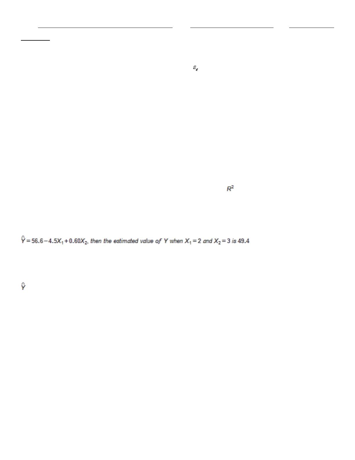
1. In a simple regression analysis, if the standard error of estimate = 15 and the number of observations n = 10, then
the sum of the residuals squared must be 120.
a.
True
b.
False
2. The adjusted R2 is used primarily to monitor whether extra explanatory variables really belong in a multiple regression
model
a.
True
b.
False
3. Correlation is used to determine the strength of the linear relationship between an explanatory variable X and response
variable Y.
a.
True
b.
False
4. In a simple linear regression problem, if the percentage of variation explained is 0.95, this means that 95% of the
variation in the explanatory variable X can be explained by regression.
a.
True
b.
False
5. In a multiple regression problem with two explanatory variables if, the fitted regression equation is
.
a.
True
b.
False
6. A regression analysis between weight (Y in pounds) and height (X in inches) resulted in the following least squares line:
= 140 + 5X. This implies that if the height is increased by 1 inch, the weight is expected to increase on average by 5
pounds.
a.
True
b.
False
7. In every regression study there is a single variable that we are trying to explain or predict. This is called the response
variable or dependent variable.
a.
True
b.
False
8. The residual is defined as the difference between the actual and predicted, or fitted values of the response variable.
a.
True
b.
False
9. A constant elasticity, or multiplicative, model the dependent variable is expressed as a product of explanatory variables
raised to powers
a.
True
Name:
Class:
Date:
chapter 10
b.
False
10. The regression line = 3 + 2X has been fitted to the data points (4, 14), (2, 7), and (1, 4). The sum of the residuals
squared will be 8.0.
a.
True
b.
False
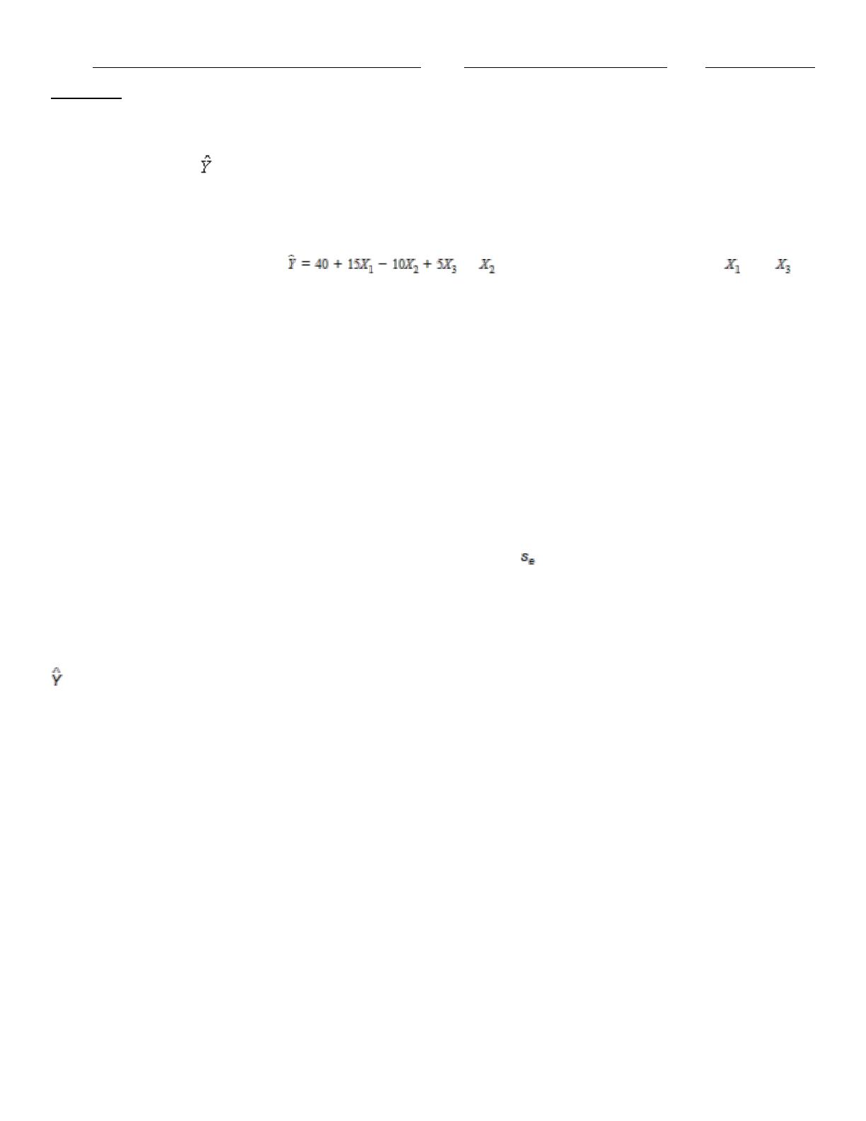
11. For the multiple regression model , if were to increase by 5 units, holding and
constant, the value of Y would be expected to decrease by 50 units.
a.
True
b.
False
12. In a simple regression with a single explanatory variable, the multiple R is the same as the standard correlation
between the Y variable and the explanatory X variable.
a.
True
b.
False
13. The effect of a logarithmic transformation on a variable that is skewed to the right by a few large values is to “squeeze”
the values together and make the distribution more symmetric
a.
True
b.
False
14. In simple linear regression, the divisor of the standard error of estimate is n – 1; simply because there is only one
explanatory variable of interest.
a.
True
b.
False
15. A regression analysis between sales (in $1000) and advertising (in $100) resulted in the following least squares line:
= 84 +7X. This implies that if advertising is $800, then the predicted amount of sales (in dollars) is $140,000.
a.
True
b.
False
16. Regression analysis can be applied equally well to cross-sectional and time series data.
a.
True
b.
False
17. Cross-sectional data are usually data gathered from approximately the same period of time from a cross-sectional of a
population.
a.
True
b.
False
18. In a nonlinear transformation of data, the Y variable or the X variables may be transformed, but not both.
a.
True
b.
False
19. To help explain or predict the response variable in every regression study, we use one or more explanatory variables.
These variables are also called response variables or independent variables.
Name:
Class:
Date:
chapter 10
a.
True
b.
False
20. When the scatterplot appears as a shapeless swarm of points, this can indicate that there is no relationship between
the response variable Y and the explanatory variable X, or at least none worth pursuing.
a.
True
b.
False
21. The multiple R for a regression is the correlation between the observed Y values and the fitted Y values.
a.
True
b.
False
22. In a multiple regression analysis with three explanatory variables, suppose that there are 60 observations and the sum
of the residuals squared is 28. The standard error of estimate must be 0.7071.
a.
True
b.
False
23. A regression analysis between sales (in $1000) and advertising (in $) resulted in the following least squares line: =
32 + 8X. This implies that an increase of $1 in advertising is expected to result in an increase of $40 in sales.
a.
True
b.
False
24. The adjusted R2 is adjusted for the number of explanatory variables in a regression equation, and it has the same
interpretation as the standard R2.
a.
True
b.
False
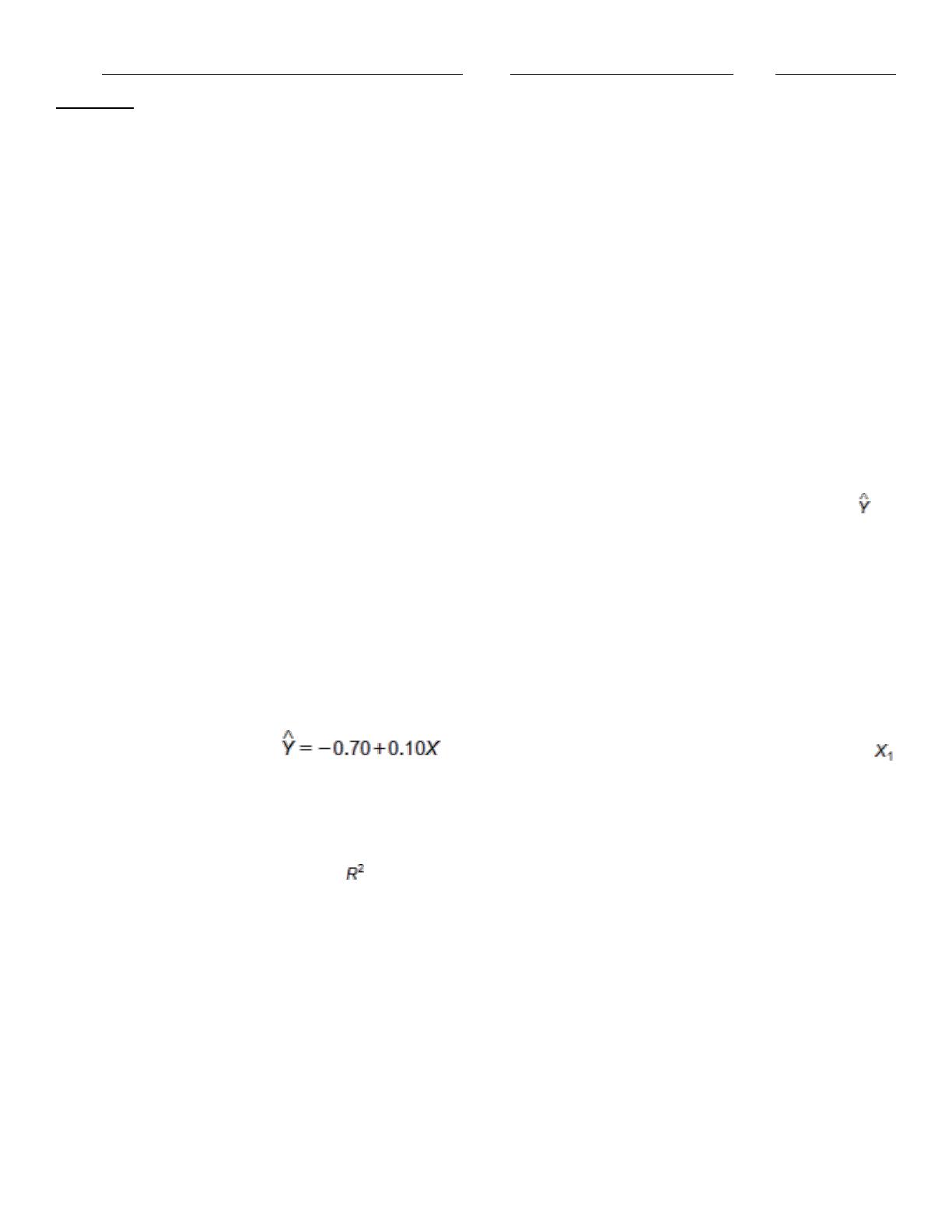
25. In reference to the equation, , the value 0.10 is the expected change in Y per unit change in
.
a.
True
b.
False
26. The percentage of variation explained is the square of the correlation between the observed Y values and the fitted
Y values.
a.
True
b.
False
27. Scatterplots are used for identifying outliers and quantifying relationships between variables.
a.
True
b.
False
28. An outlier is an observation that falls outside of the general pattern of the rest of the observations on a scatterplot.
a.
True
b.
False
Name:
Class:
Date:
chapter 10
29. In regression analysis, we can often use the standard error of estimate to judge which of several potential
regression equations is the most useful.
a.
True
b.
False
30. The least squares line is the line that minimizes the sum of the residuals.
a.
True
b.
False
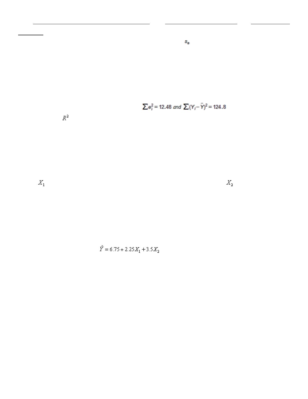
31. In a simple linear regression problem, suppose that . Then the percentage of
variation explained must be 0.90.
a.
True
b.
False
32. An interaction variable is the product of an explanatory variable and the dependent variable.
a.
True
b.
False
33. We should include an interaction variable in a regression model if we believe that the effect of one explanatory
variable on the response variable Y depends on the value of another explanatory variable .
a.
True
b.
False
34. The coefficients for logarithmically transformed explanatory variables should be interpreted as the percent change in
the dependent variable for a 1% percent change in the explanatory variable.
a.
True
b.
False
35. In the multiple regression model we interpret X1 as follows: holding X2 constant, if X1
increases by 1 unit, then the expected value of Y will increase by 9 units.
a.
True
b.
False
36. If the regression equation includes anything other than a constant plus the sum of products of constants and variables,
the model will not be linear
a.
True
b.
False
37. A logarithmic transformation of the response variable Y is often useful when the distribution of Y is symmetric.
a.
True
b.
False
38. Correlation is measured on a scale from 0 to 1, where 0 indicates no linear relationship between two variables, and 1
indicates a perfect linear relationship.
a.
True
b.
False

Name:
Class:
Date:
chapter 10
39. A useful graph in almost any regression analysis is a scatterplot of residuals (on the vertical axis) versus fitted values
(on the horizontal axis), where a “good” fit not only has small residuals, but it has residuals scattered randomly around
zero with no apparent pattern.
a.
True
b.
False
40. If a categorical variable is to be included in a multiple regression, a dummy variable for each category of the variable
should be used, but the original categorical variables should not be sued.
a.
True
b.
False
41. A negative relationship between an explanatory variable X and a response variable Y means that as X increases, Y
decreases, and vice versa.
a.
True
b.
False
42. A regression analysis between sales (in $1000) and advertising (in $100) resulted in the following least squares line:
= 84 +7X. This implies that if there is no advertising, then the predicted amount of sales (in dollars) is $84,000.
a.
True
b.
False
43. The primary purpose of a nonlinear transformation is to “straighten out” the data on a scatterplot
a.
True
b.
False
44. If a scatterplot of residuals shows a parabola shape, then a logarithmic transformation may be useful in obtaining a
better fit
a.
True
b.
False
45. The two primary objectives of regression analysis are to study relationships between variables and to use those
relationships to make predictions.
a.
True
b.
False
46. The R2 can only increase when extra explanatory variables are added to a multiple regression model
a.
True
b.
False
Indicate the answer choice that best completes the statement or answers the question.
47. A scatterplot that appears as a shapeless mass of data points indicates:
a.
a curved relationship among the variables
b.
a linear relationship among the variables
c.
a nonlinear relationship among the variables
d.
no relationship among the variables
Name:
Class:
Date:
chapter 10
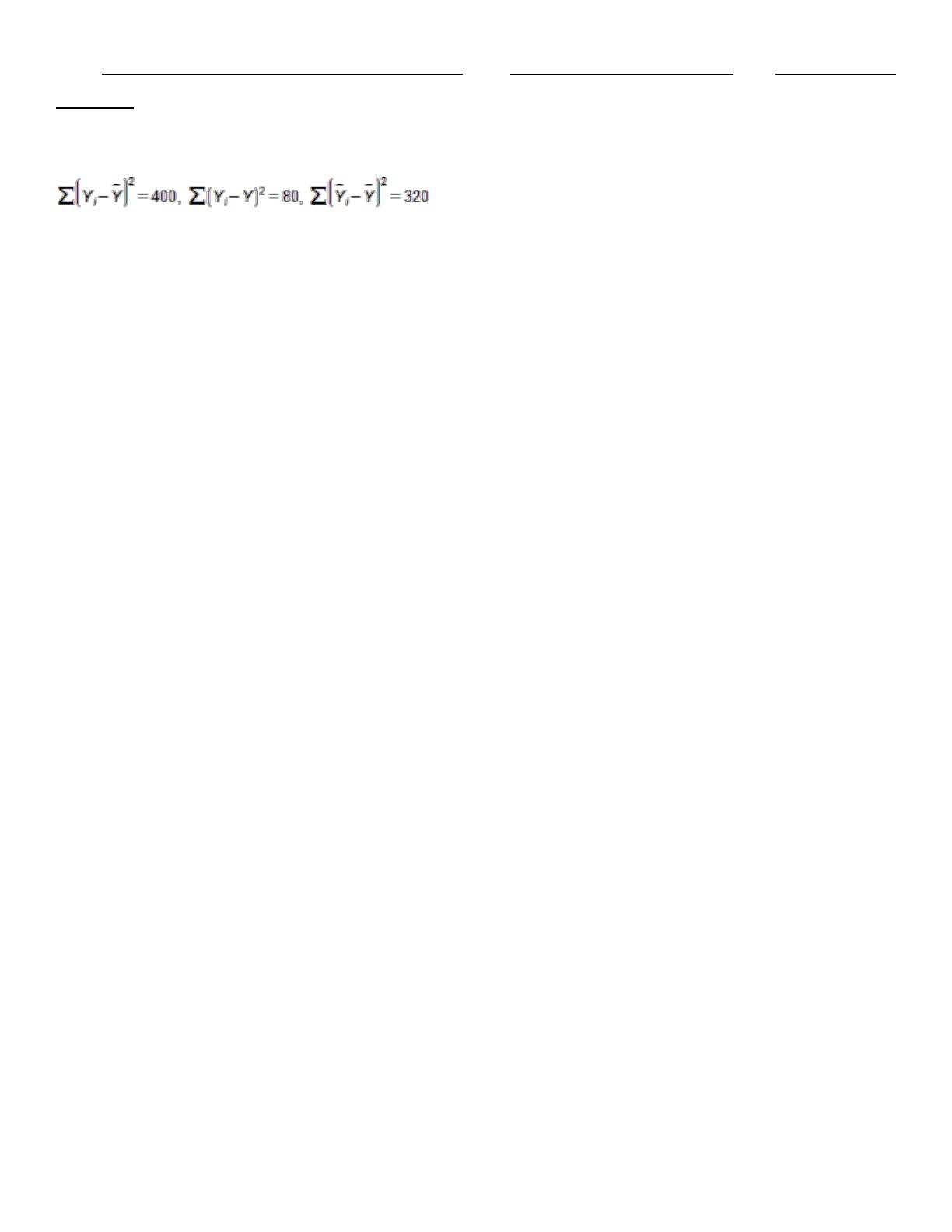
48. In a simple linear regression analysis, the following sums of squares are produced:
The proportion of the variation in Y that is explained by the variation in X is:
a.
20%
b.
80%
c.
25%
d.
50%
e.
None of the above
49. The covariance is not used as much as the correlation because
a.
is not always a valid predictor of linear relationships
b.
it is difficult to calculate
c.
it is difficult to interpret
d.
all of these options
50. In regression analysis, if there are several explanatory variables, it is called:
a.
simple regression
b.
multiple regression
c.
compound regression
d.
composite regression
51. A single variable X can explain a large percentage of the variation in some other variable Y when the two variables
are:
a.
mutually exclusive
b.
inversely related
c.
directly related
d.
highly correlated
e.
None of the above
52. The adjusted R2 adjusts R2 for:
a.
non-linearity
b.
outliers
c.
low correlation
d.
the number of explanatory variables in a multiple regression model
53. In regression analysis, which of the following causal relationships are possible?
a.
X causes Y to vary
b.
Y causes X to vary
c.
Other variables cause both X and Y to vary
d.
All of these options
Name:
Class:
Date:
chapter 10
54. The regression line has been fitted to the data points (28, 60), (20, 50), (10, 18), and (25, 55). The sum
of the squared residuals will be:
a.
20.25
b.
16.00
c.
49.00
d.
94.25
55. In regression analysis, the variable we are trying to explain or predict is called the
a.
independent variable
b.
dependent variable
c.
regression variable
d.
statistical variable
e.
residual variable
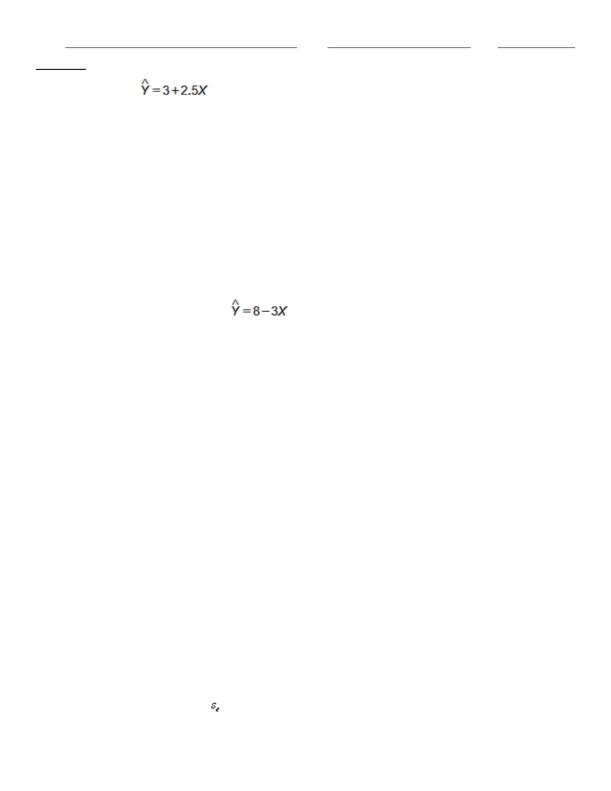
56. Given the least squares regression line,
a.
the relationship between X and Y is positive
b.
the relationship between X and Y is negative
c.
as X increases, so does Y
d.
as X decreases, so does Y
e.
there is no relationship between X and Y
57. The correlation value ranges from
a.
0 to +1
b.
–1 to +1
c.
–2 to +2
d.
-Y to +Y
58. In linear regression, we can have an interaction variable. Algebraically, the interaction variable is the other variables in
the regression equation.
a.
sum
b.
ratio
c.
product
d.
mean
59. A correlation value of zero indicates.
a.
a strong linear relationship
b.
a weak linear relationship
c.
no linear relationship
d.
a perfect linear relationship
60. The standard error of the estimate ( ) is essentially the
a.
mean of the residuals
b.
standard deviation of the residuals

Name:
Class:
Date:
chapter 10
c.
mean of the explanatory variable
d.
standard deviation of the explanatory variable
61. A “fan” shape in a scatterplot indicates:
a.
unequal variance
b.
a nonlinear relationship
c.
the absence of outliers
d.
sampling error
62. In multiple regression, the coefficients reflect the expected change in:
a.
Y when the associated X value increases by one unit
b.
X when the associated Y value increases by one unit
c.
Y when the associated X value decreases by one unit
d.
X when the associated Y value decreases by one unit
63. Correlation is a summary measure that indicates:
a.
a curved relationship among the variables
b.
the rate of change in Y for a one unit change in X
c.
the strength of the linear relationship between pairs of variables
d.
the magnitude of difference between two variables
64. An important condition when interpreting the coefficient for a particular independent variable X in a multiple regression
equation is that:
a.
the dependent variable will remain constant
b.
the dependent variable will be allowed to vary
c.
all of the other independent variables remain constant
d.
all of the other independent variables be allowed to vary
65. The percentage of variation ( ) can be interpreted as the fraction (or percent) of variation of the
a.
explanatory variable explained by the independent variable
b.
explanatory variable explained by the regression line
c.
response variable explained by the regression line
d.
error explained by the regression line
66. In linear regression, the fitted value is the:
a.
predicted value of the dependent variable
b.
predicted value of the independent value
c.
predicted value of the slope
d.
predicted value of the intercept
e.
None of these options
67. In regression analysis, the variables used to help explain or predict the response variable are called the
a.
independent variables
b.
dependent variables
c.
regression variables

Name:
Class:
Date:
chapter 10
d.
statistical variables
68. Approximately what percentage of the observed Y values are within one standard error of the estimate of the
corresponding fitted Y values?
a.
67%
b.
95%
c.
99%
d.
It is not possible to say
69. In linear regression, we fit the least squares line to a set of values (or points on a scatterplot). The distance from the
line to a point is called the:
a.
fitted value
b.
residual
c.
correlation
d.
covariance
e.
None of these options
70. In choosing the “best–fitting” line through a set of points in linear regression, we choose the one with the:
a.
smallest sum of squared residuals
b.
largest sum of squared residuals
c.
smallest number of outliers
d.
largest number of points on the line
e.
None of these options
71. The weakness of scatterplots is that they:
a.
do not help identify linear relationships
b.
can be misleading about the types of relationships they indicate
c.
only help identify outliers
d.
do not actually quantify the relationships between variables
72. is/are especially helpful in identifying outliers.
a.
Linear regression
b.
Regression analysis
c.
Normal curves
d.
Scatterplots
e.
Multiple regression
73. Regression analysis asks:
a.
if there are differences between distinct populations
b.
if the sample is representative of the population
c.
how a single variable depends on other relevant variables
d.
how several variables depend on each other
74. The term autocorrelation refers to:
a.
the analyzed data refers to itself

Name:
Class:
Date:
chapter 10
b.
the sample is related too closely to the population
c.
the data are in a loop (values repeat themselves)
d.
time series variables are usually related to their own past values
75. A multiple regression analysis including 50 data points and 5 independent variables results in 40. The multiple
standard error of estimate will be:
a.
0.901
b.
0.888
c.
0.800
d.
0.953
e.
0.894
76. Outliers are observations that
a.
lie outside the sample
b.
render the study useless
c.
lie outside the typical pattern of points on a scatterplot
d.
disrupt the entire linear trend
77. In linear regression, a dummy variable is used:
a.
to represent residual variables
b.
to represent missing data in each sample
c.
to include hypothetical data in the regression equation
d.
to include categorical variables in the regression equation
e.
when “dumb” responses are included in the data
78. The percentage of variation (R2) ranges from
a.
0 to +1
b.
–1 to +1
c.
–2 to +2
d.
–1 to 0
79. Data collected from approximately the same period of time from a cross-section of a population are called:
a.
time series data
b.
linear data
c.
cross-sectional data
d.
historical data
80. In multiple regression, the constant :
a.
Is the expected value of the dependent variable Y when all of the independent variables have the value zero
b.
Is necessary to fit the multiple regression line to set of points
c.
Must be adjusted for the number of independent variables
d.
All of these options
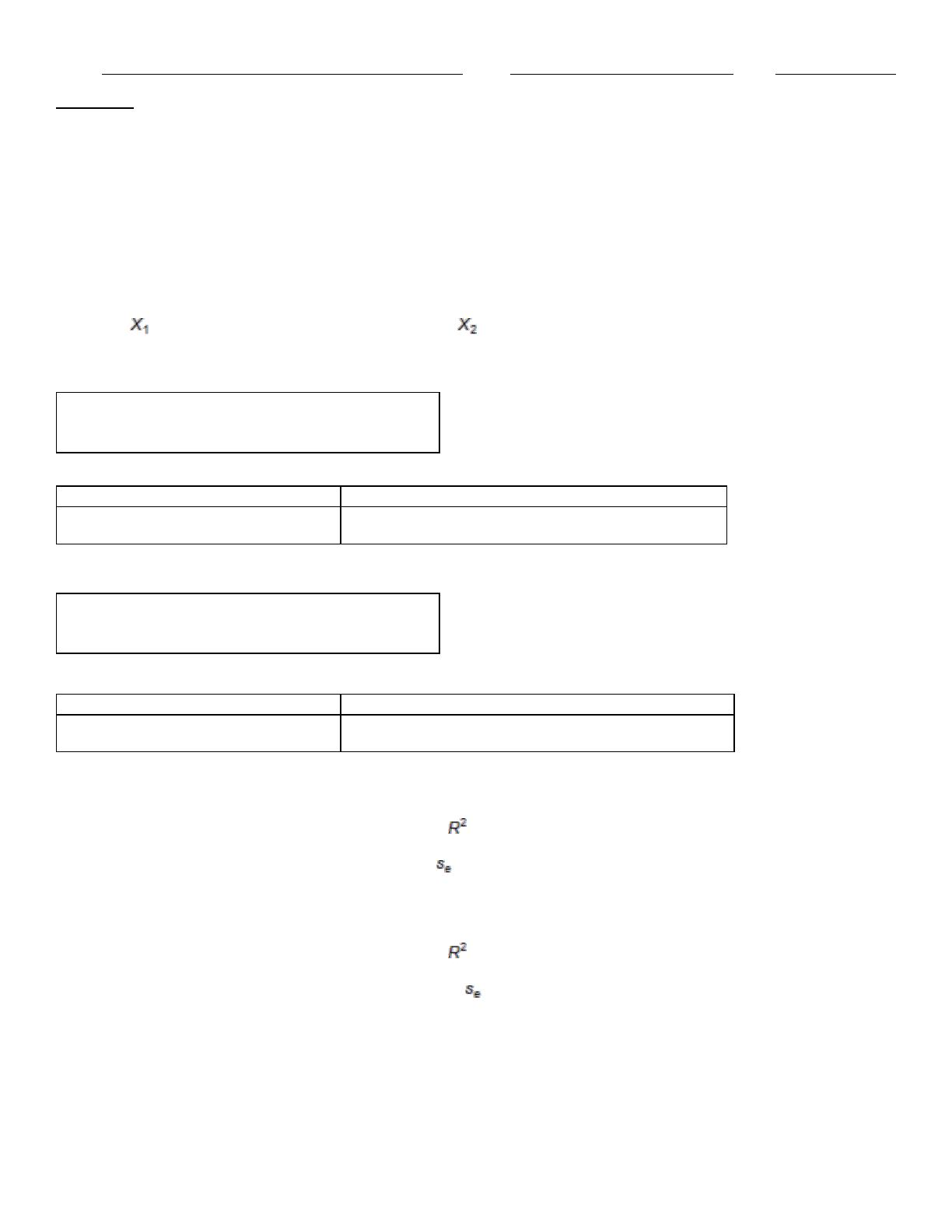
81. Which of the following is an example of a nonlinear regression model?
Name:
Class:
Date:
chapter 10
a.
A quadratic regression equation
b.
A logarithmic regression equation
c.
Constant elasticity equation
d.
The learning curve model
e.
All of these options
The information below represents the relationship between the selling price (Y, in $1000) of a home, the square footage of
the home ( ), and the number of bedrooms in the home ( ). The data represents 65 homes sold in a particular area of
a city and was analyzed using simple linear regression for each independent variable.
Summary measures
Multiple R
0.8148
R-Square
0.6640
StErr of Estimate
8.5572
Regression coefficients
Coefficient
Std Err
t-value
p-value
Constant
52.157
7.4784
6.9744
0.0000
Square Footage
4.646
0.4164
11.1575
0.0000
Summary measures
Multiple R
0.6487
R-Square
0.4208
StErr of Estimate
11.2344
Regression coefficients
Coefficient
Std Err
t-value
p-value
Constant
100.628
5.2324
19.2316
0.0000
Number of Bedrooms
11.035
1.6310
6.7660
0.0000
82. (A) Is there evidence of a linear relationship between the selling price and the square footage of the homes? If so,
interpret the least squares line and characterize the relationship (i.e., positive, negative, strong, weak, etc.).
(B) Identify and interpret the coefficient of determination ( ) for the model in (A).
(C) Identify and interpret the standard error of estimate for the model in (A).
(D) Is there evidence of a linear relationship between the selling price and number of bedrooms of the homes? If so,
interpret the least squares line and characterize the relationship (i.e., positive, negative, strong, weak, etc.).
(E) Identify and interpret the coefficient of determination ( ) for the model in (D).
(F) Identify and interpret the standard error of the estimate ( ) for the model in (C).
(G) Which of the two variables, the square footage or the number of bedrooms, is the relationship with home selling price
stronger? Justify your choice.
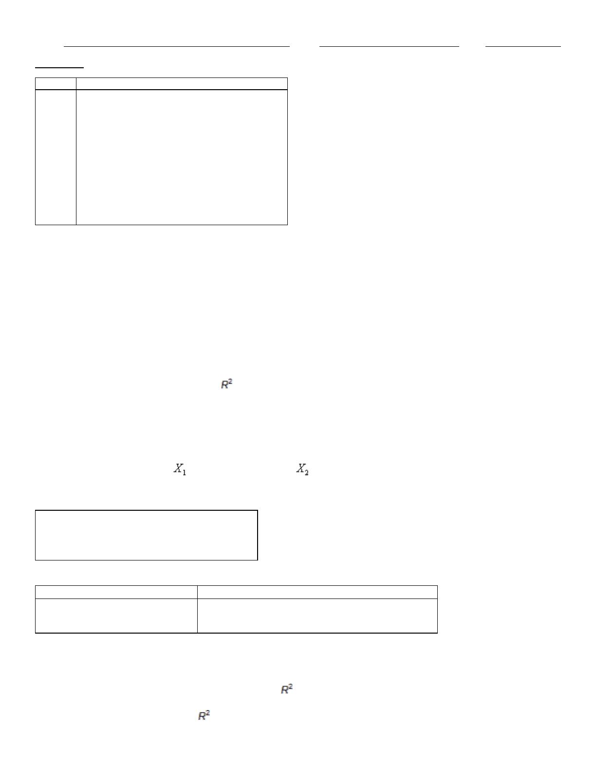
The marketing manager of a large supermarket chain would like to determine the effect of shelf space (in feet) on the
weekly sales of international food (in hundreds of dollars). A random sample of 12 equal –sized stores is selected, with
the following results:
Name:
Class:
Date:
chapter 10
Store
Shelf Space X
Weekly Sales Y
1
10
2.0
2
10
2.6
3
10
1.8
4
15
2.3
5
15
2.8
6
15
3.0
7
20
2.7
8
20
3.1
9
20
3.2
10
25
3.0
11
25
3.3
12
25
3.5
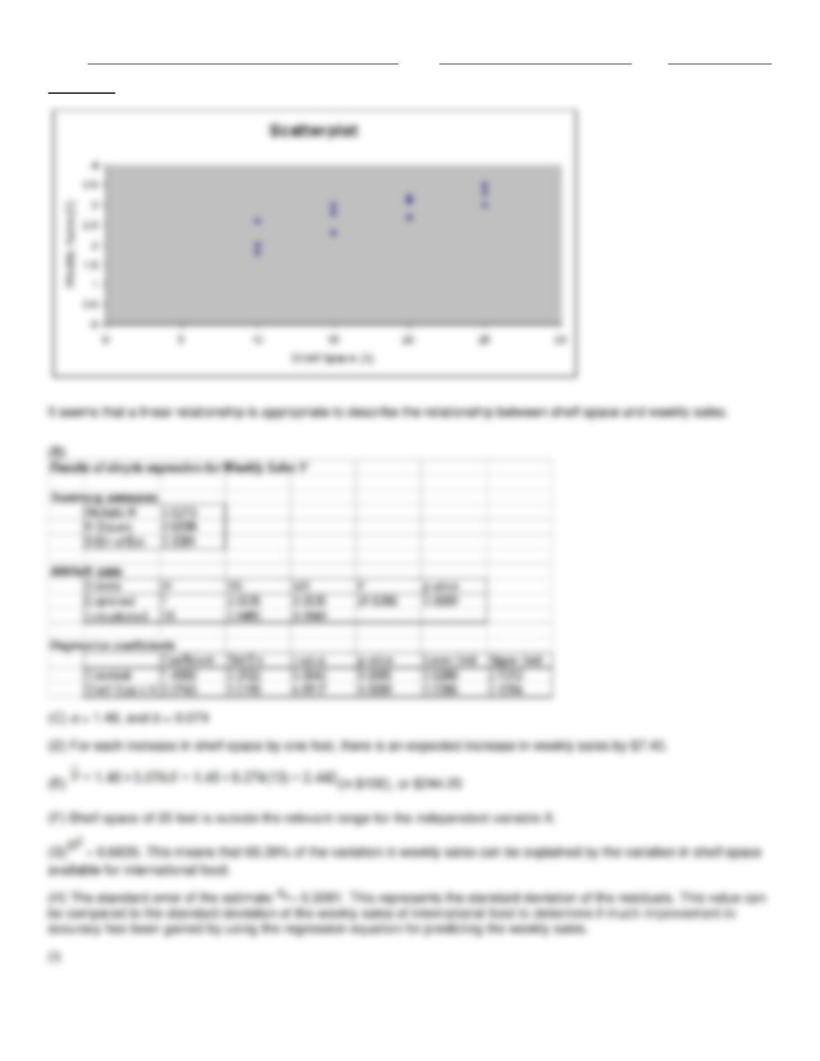
83. (A) Draw a scatterplot of the data and comment on the relationship between shelf space and weekly sales.
(B) Run a regression on this data set and report the results.
(C) What are the least squares regression coefficients of the Y-intercept (a) and slope (b)?
(D) Interpret the meaning of the slope b.
(E) Predict the average weekly sales (in hundreds of dollars) of international food for stores with 13 feet of shelf space for
international food.
(F) Why would it not be appropriate to predict the average weekly sales (in hundreds of dollars) of international food for
stores with 35 feet of shelf space for international food?
(G) Identify the coefficient of determination, , and interpret its meaning.
(H) Determine the standard error of the estimate. What does it represent?
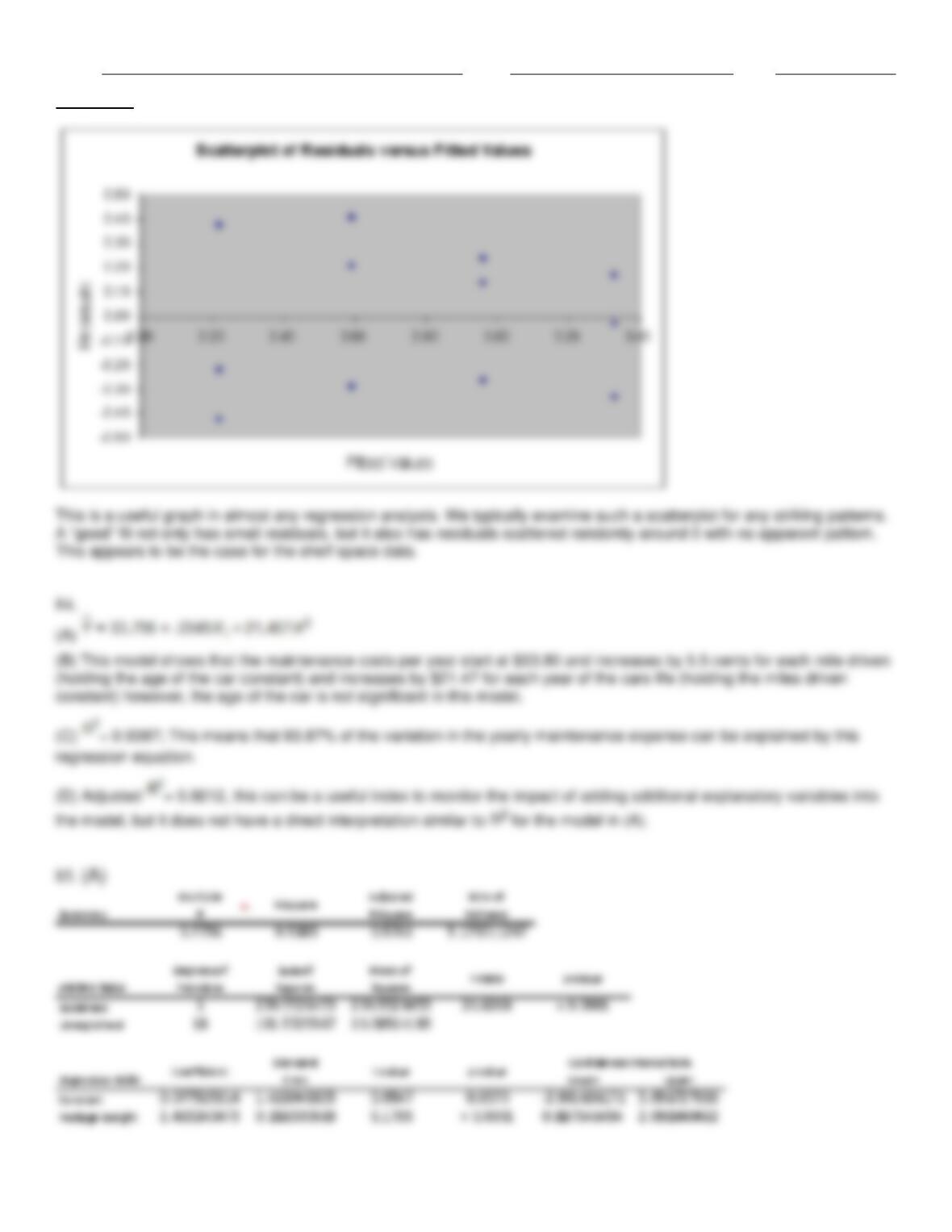
(I) Draw a scatterplot of residuals versus fitted values. What does this graph indicate?
An automobile rental company wants to predict the yearly maintenance expense (Y) for an automobile using the number
of miles driven during the year ( ) and the age of the car ( , in years) at the beginning of the year. The company has
gathered the data on 10 automobiles and run a regression analysis with the results shown below.
Summary measures
Multiple R
0.9689
R-Square
0.9387
Adj R-Square
0.9212
StErr of Estimate
72.218
Regression coefficients
Coefficient
Std Err
t-value
p-value
Constant
33.796
48.181
0.7014
0.5057
Miles Driven
0.0549
0.0191
2.8666
0.0241
Age of car
21.467
20.573
1.0434
0.3314
84. (A) Use the information above to estimate the linear regression model.
(B) Interpret each of the estimated regression coefficients of the regression model in (A).
(C) Identify and interpret the coefficient of determination ( ), for the model in (A).
(D) Identify and interpret the adjusted for the model in (A).
Name:
Class:
Date:
chapter 10
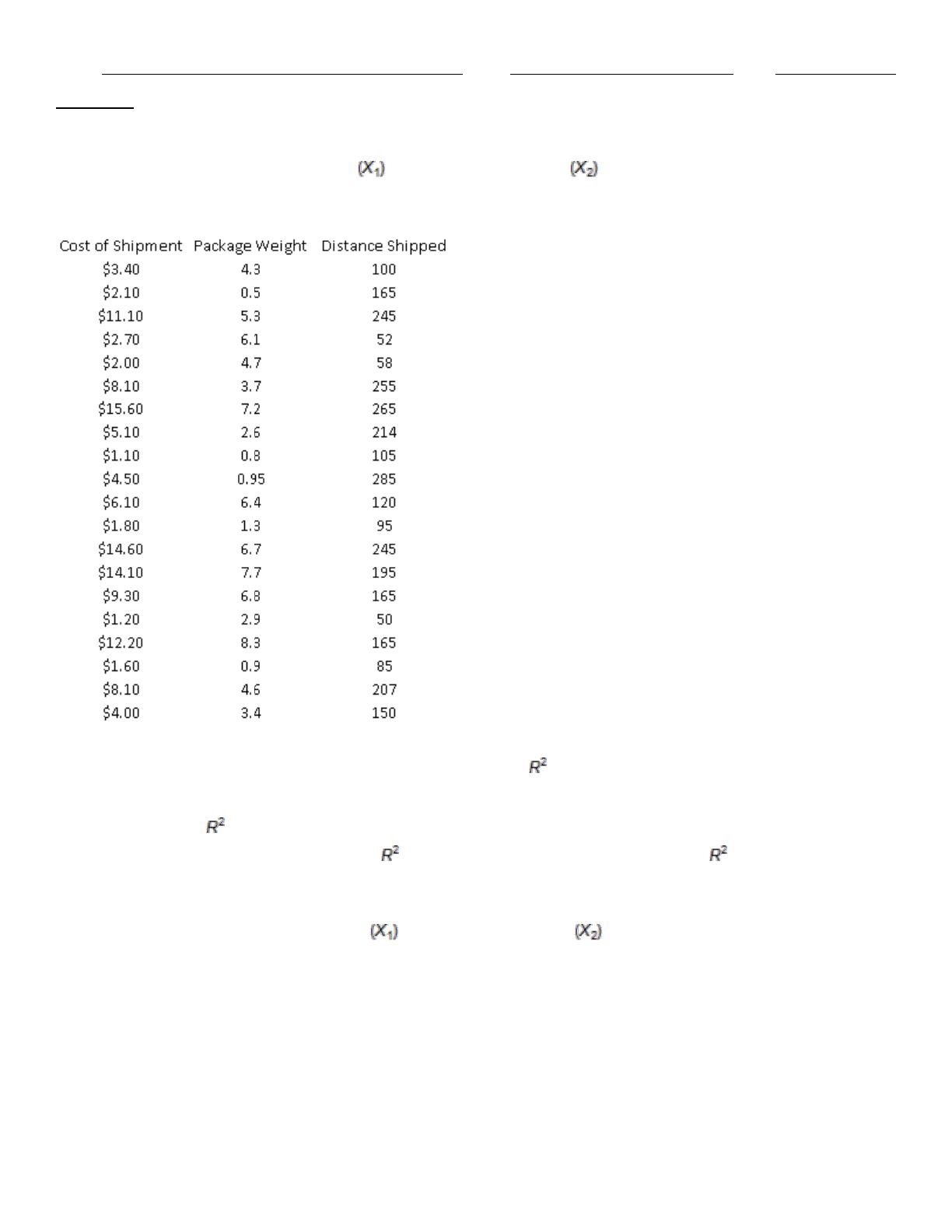
An express delivery service company recently conducted a study to investigate the relationship between the cost of
shipping a package (Y), the package weight , and the distance shipped . Twenty packages were randomly
selected from among the large number received for shipment, and a detailed analysis of the shipping cost was conducted
for each package. The sample information is shown in the table below:
85. (A) Estimate a simple linear regression model involving shipping cost and package weight. Interpret the slope
coefficient of the least squares line as well as the computed value of .
(B) Add another explanatory variable – distance shipped – to the regression to (A). Estimate and interpret this expanded
model. How does the value for this multiple regression model compare to that of the simple regression model estimated
in (A)? Explain any difference between the two values. Compute and interpret the adjusted value for the revised
model.
(C) Suppose that one of the managers of this express delivery service company is trying to decide whether to add an
interaction term involving the package weight and the distance shipped in the multiple regression model
developed previously. Why would the manager want to add such a term to the regression equation?
(D) Estimate the revised model using the interaction term suggested in (C).
(E) Interpret each of the estimated coefficients in your revised model in (D). In particular, how do you interpret the
coefficient for the interaction term in the revised model?
(F) Does this revised model in (D) fit the given data better than the original multiple regression model in (B)? Explain why
or why not.
A large auto dealership is interested in determining the number of cars that will be sold in a given quarter. The
management of the dealership believes that a relationship can be found between the number of cars sold (Y), the
Name:
Class:
Date:
chapter 10
advertised price ( ) and the current interest rates ( ). Their past experience shows that they tend to have better luck
using a non-linear relationship. Below is the output from a regression analysis using the natural logarithm of the variables
in the model.
Summary measures
Multiple R
0.9326
R-Square
0.8698
Adj R-Square
0.8498
StErr of Estimate
0.0259
ANOVA Table
Source
df
SS
MS
F
p-value
Explained
2
0.0581
0.0290
43.4187
0.0000
Unexplained
13
0.0087
0.0007
Regression coefficients
Coefficient
Std Err
t-value
p-value
Constant
4.3965
0.7549
5.8239
0.0001
Log Price
-0.8255
0.2467
3.3456
0.0053
Log Interest
-0.1225
0.1880
-0.6512
0.5262
86. (A) Use the information above to estimate the regression model.
(B) Interpret each of the estimated regression coefficients of the regression model in (A).
(C) Does using a non-linear model seem to be a good choice in this example? Explain your answer.
The station manager of a local television station is interested in predicting the amount of television (in hours) that people
will watch in the viewing area. The explanatory variables are: age (in years), education (highest level obtained, in
years) and family size (number of family members in household). The multiple regression output is shown below:
Summary measures
Multiple R
0.8440
R-Square
0.7123
Adj R-Square
0.6644
StErr of Estimate
0.5598
ANOVA Table
Source
df
SS
MS
F
p-value
Explained
3
13.9682
4.6561
14.8564
0.0000
Unexplained
18
5.6413
0.3134
Regression coefficients
Coefficient
Std Err
t-value
p-value
Constant
1.683
1.1696
1.4389
0.1674
Age
-0.0498
0.0199
-2.5018
0.0222
Education
0.2135
0.0503
4.2426
0.0005
Family Size
0.0405
0.0784
0.5168
0.6116
87. (A) Use the information above to estimate the linear regression model.
(B) Interpret each of the estimated regression coefficients of the regression model in (A).
(C) Identify and interpret the coefficient of determination ( ) for the model in (A).
Name:
Class:
Date:
chapter 10
(D) Identify and interpret the standard error of the estimate for the model in (A).
The human resource manager at Gamma, Inc. wants to examine the relationship between annual salaries (Y), the number
of years employees have worked at Gamma, Inc. ( ) and whether the employee is male or female ( ). They are also
interested in whether the interaction between the two explanatory variables ( ) has a significant impact on salaries.
These data have been collected for a sample of 28 employees and the regression output is shown below.
Summary measures
Multiple R
0.8065
R-Square
0.6504
Adj R-Square
0.6067
StErr of Estimate
6572.3
Regression coefficients
Coefficient
Std Err
t-value
p-value
Constant
29831.68
3904.56
7.640
0.0000
Years Employed
869.04
266.78
3.258
0.0033
Gender
-2396.54
4620.04
–0.519
0.6087
Years & Gender
403.93
350.38
1.153
0.2603
88. (A) Use the information above to estimate the linear regression model.
(B) Write the regression equation in (A) as two separate equations; one for females and one for males, and interpret the
results.
(C) Would any of the variables in the linear regression model in (A) be considered a dummy variable? Explain your
answer.
(D) Identify and interpret the coefficient of determination ( ) for the model in (A).
(E) Identify and interpret the standard error of estimate (se) for the model in (A).
A new online auction site specializes in selling automotive parts for classic cars. The founder of the company believes that
the price received for a particular item increases with its age (i.e., the age of the car on which the item can be used in
years) and with the number of bidders. The multiple regression output is shown below.
Summary measures
Multiple R
0.8391
R-Square
0.7041
Adj R-Square
0.6783
StErr of Estimate
148.828
Regression coefficients
Coefficient
Std Err
t-value
p-value
Constant
-1242.986
331.204
-3.7529
0.0010
Age of part
75.017
10.647
7.0459
0.0000
Number of Bidders
13.973
10.443
1.3380
0.1940
89. (A) Use the information above to estimate the linear regression model.
(B) Interpret each of the estimated regression coefficients of the regression model in (A).
(C) Identify and interpret the coefficient of determination ( ) for the model in (A).
Name:
Class:
Date:
chapter 10
(D) Identify and interpret the standard error of the estimate (se) for the model in (A).
(E) Would you recommend that this company examine any other factors to predict the selling price? If yes, what other
factors would you want to consider? Explain your answer.
La Cabaña, a popular motel chain in the southwest, is interested in developing a regression model that can predict the
occupancy rate (%) of its motels. Currently, the company is interested in using two explanatory variables to predict
occupancy. They want to use the amount of advertising (in $) used by each motel and if the particular location a
franchised location. Some regression information is presented below:
Summary measures
Multiple R
0.5358
R-Square
0.2871
Adj R-Square
0.2223
StErr of Estimate
7.582
Regression coefficients
Coefficient
Std Err
t-value
p-value
Constant
43.118
11.4263
3.7735
0.0010
Advertising
0.0013
0.0006
2.4119
0.0247
Franchise
3.038
3.1759
0.9567
0.3491
90. (A) Use the information above to estimate the linear regression model.
(B) Interpret each of the estimated regression coefficients of the regression model in (A).
(C) Would any of the variables in this model be considered a dummy variable? Explain your answer.
(D) Identify and interpret the coefficient of determination ( ) and the standard error of the estimate (se) for the model in
(A).
A realtor in a local area is interested in being able to predict the selling price for a newly listed home or for someone
considering listing their home. This realtor would like to attempt to predict the selling price by using the size of the home (
, in hundreds of square feet), the number of rooms ( ), the age of the home ( , in years) and if the home has an
attached garage ( ). Use the output below to determine if this realtor will be able to use this information to predict the
selling price (in $1000).
Summary measures
Multiple R
0.9439
R-Square
0.8910
Adj. R-Square
0.8474
StErr of Estimate
22.241
Regression coefficients
Coefficient
Std Err
t-value
p-value
Constant
-19.026
54.769
-0.3474
0.7355
Size
7.494
1.529
4.9010
0.0006
Number of Rooms
7.153
9.211
0.7767
0.4553
Age
–0.673
0.992
-0.6789
0.5126
Attached Garage
0.453
20.192
0.0224
0.9826
91. (A) Use the information above to estimate the linear regression model.
(B) Interpret each of the estimated regression coefficients of the regression model in (A).
Name:
Class:
Date:
chapter 10
(C) Would any of the variables in this model be considered a dummy variable? Explain your answer.
(D) Identify and interpret the coefficient of determination ( ) and the standard error of the estimate (se) for the model in
(A).
(E) Use the estimated model in (A) to predict the sales price of a 2500 square feet, 15-year old house that has 5 rooms
and an attached garage.
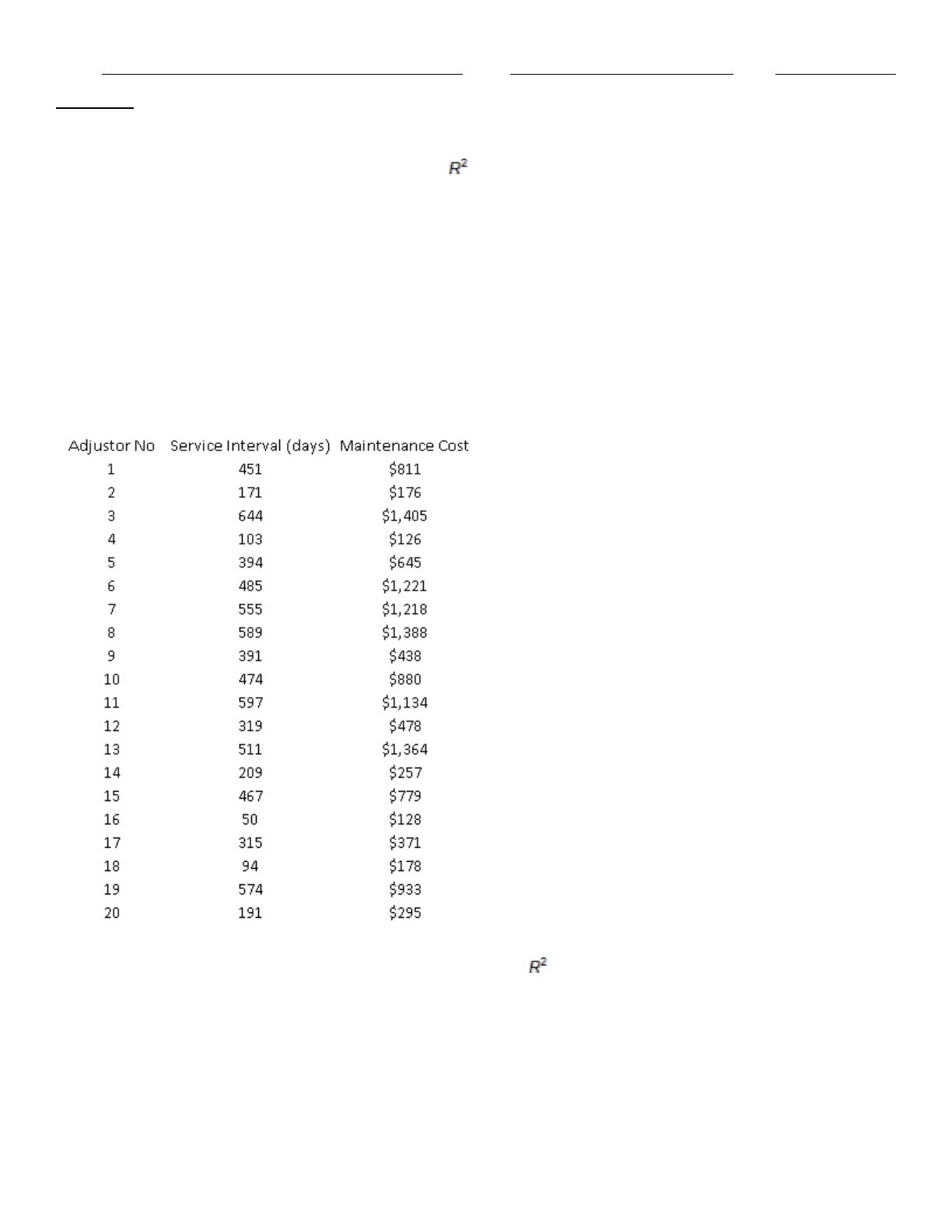
Adjustors working for a large insurance agency are each given a company car which they use on the job to travel to client
locations to inspect damage to homes and automobiles that are covered by the agency. Although the cars are owned by
the agency, maintenance is currently left up to the discretion of the adjustors, who are reimbursed for any costs they
report. The agency believes that the lack of a maintenance policy has led to unnecessary maintenance expenses. In
particular, they believe that many agents wait too long to have maintenance performed on their company cars, and that in
such cases, maintenance expenses are inordinately high. The agency recently conducted a study to investigate the
relationship between the reported cost of maintenance visits for their company cars (Y) and the length of time since the
last maintenance service (X). The sample data are shown below:
92. (A) Estimate a simple linear regression model with Service Interval (X) and Maintenance Cost (Y). Interpret the slope
coefficient of the least squares line as well as the computed value of .
(B) Do you think this model proves the agency’s point about maintenance? Explain your answer.
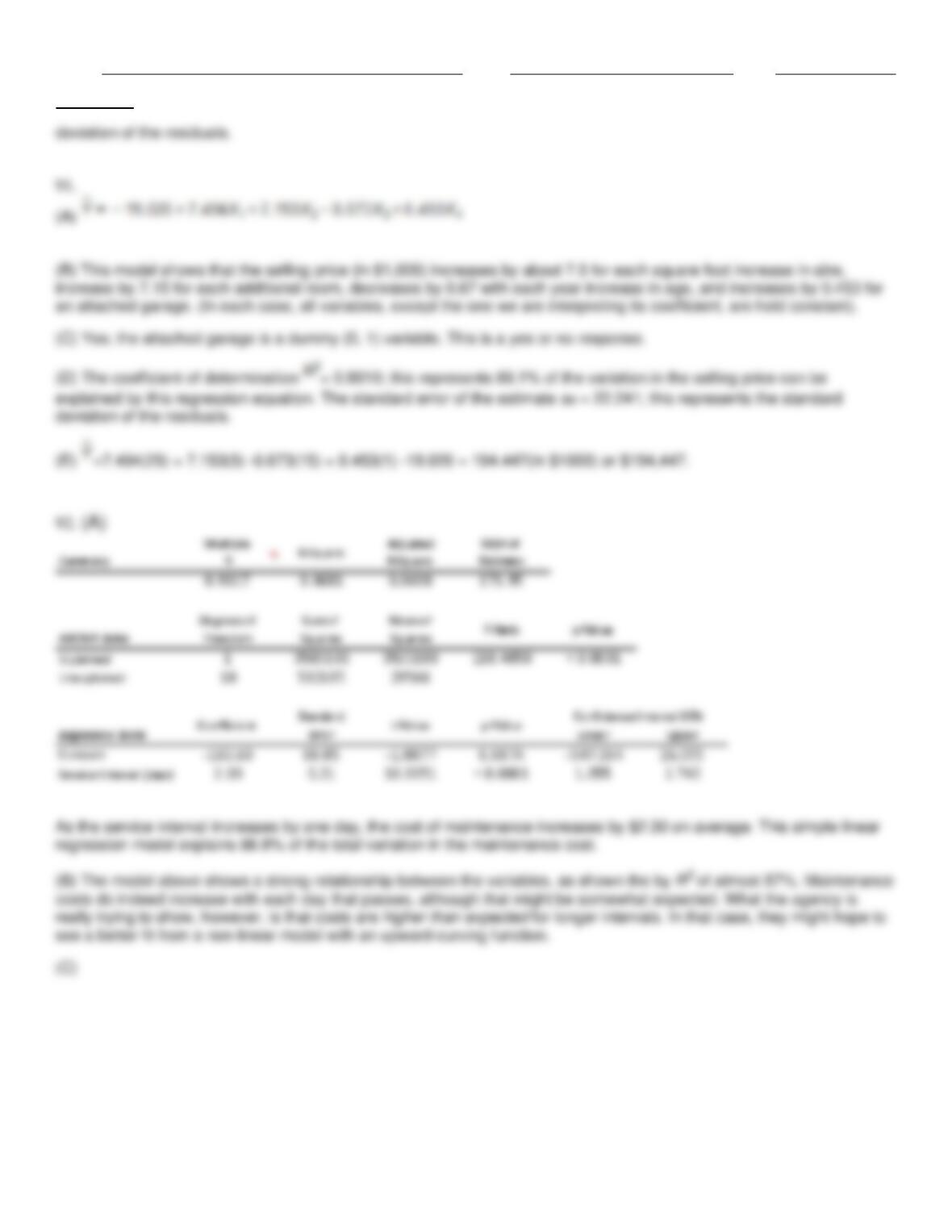
(C) Obtain a residual plot vs. Service Interval. Does this affect your opinion of the validity of the model in (A)?
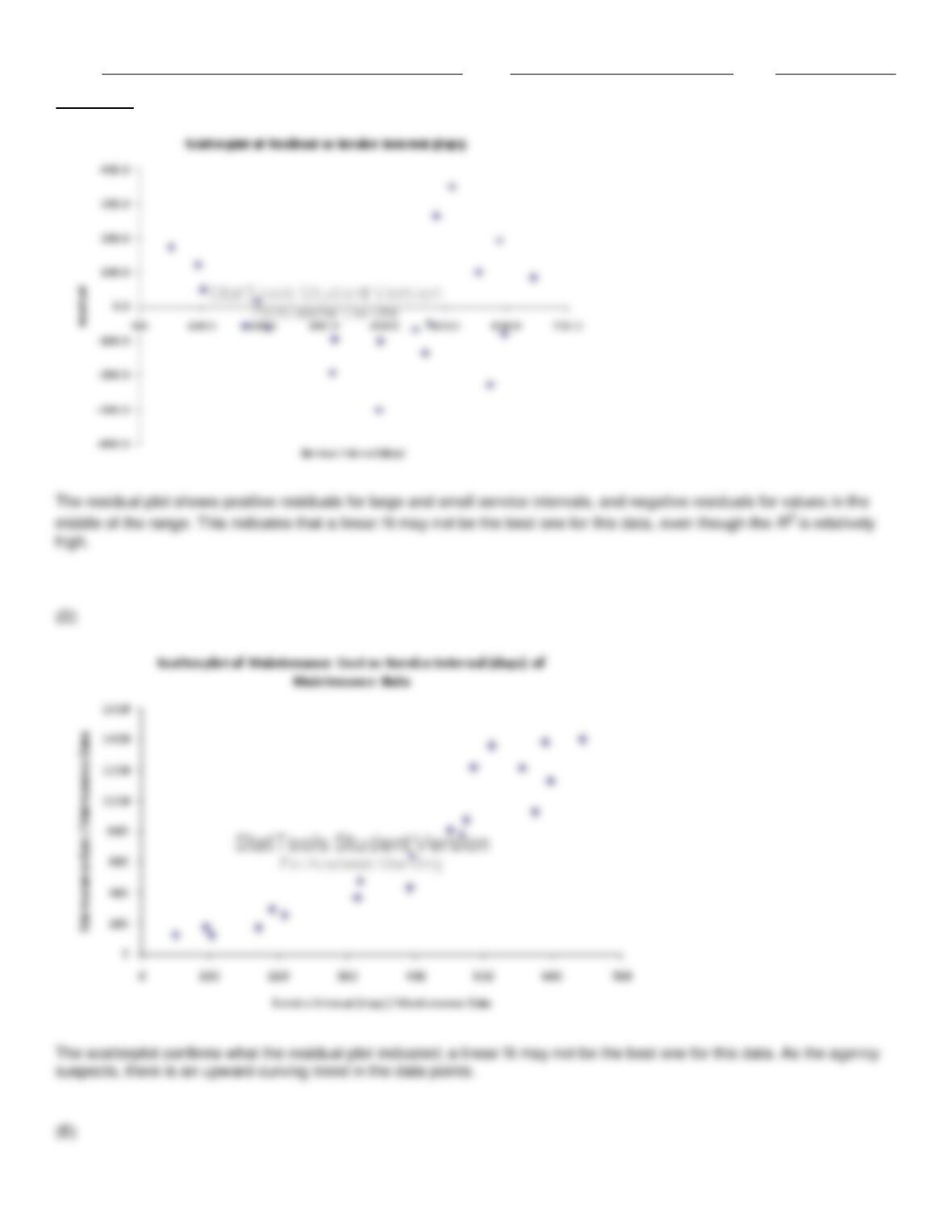
(D) Obtain a scatterplot of Maintenance Cost vs. Service Interval. Does this affect your opinion of the validity of the model
in (A)?
(E) Use what you have learned about transformations to fit an alternative model to the one in (A).

Name:
Class:
Date:
chapter 10
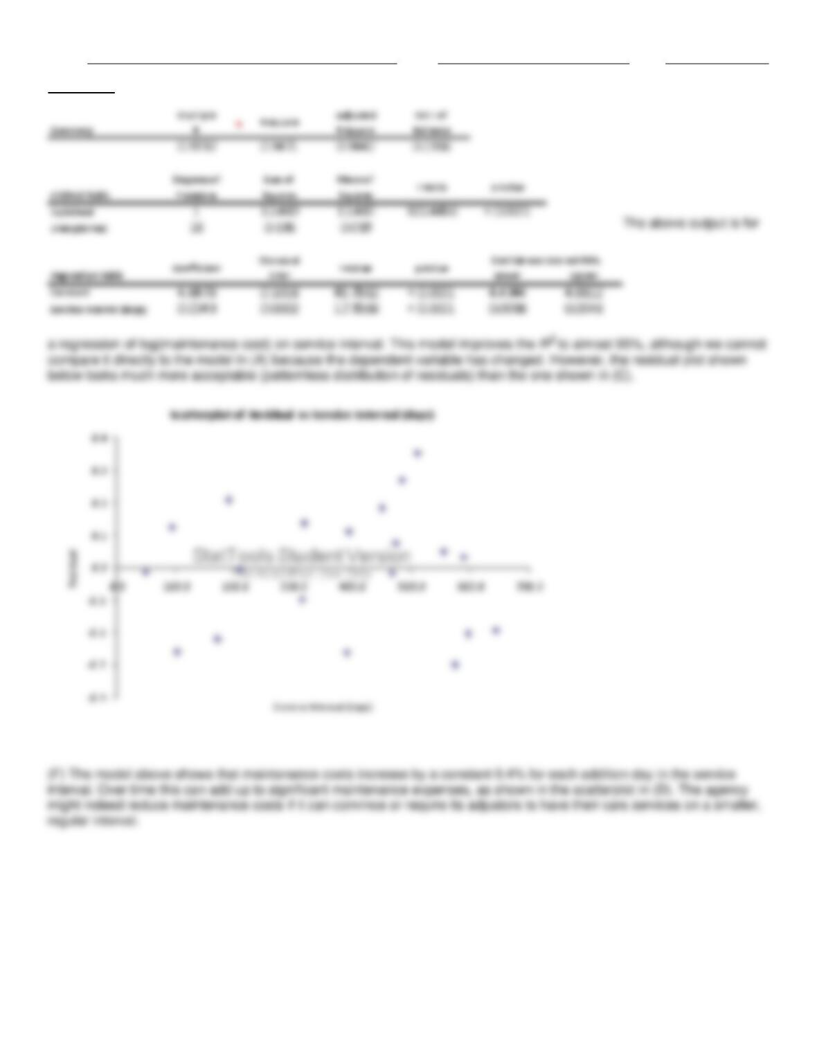
(F) Interpret the model you developed in (E). Does it help you assess the agency’s claim? What should the agency
conclude about the relationship between service interval and maintenance costs?
Name:
Class:
Date:
chapter 10
Answer Key
Name:
Class:
Date:
chapter 10
Name:
Class:
Date:
chapter 10
Name:
Class:
Date:
chapter 10
Name:
Class:
Date:
chapter 10
(I)
Name:
Class:
Date:
chapter 10
Name:
Class:
Date:
chapter 10
Name:
Class:
Date:
chapter 10
improvement in accuracy has been gained by using the regression equation to predict this expense.
Name:
Class:
Date:
chapter 10
Name:
Class:
Date:
chapter 10
Name:
Class:
Date:
chapter 10
Name:
Class:
Date:
chapter 10