In conducting the Wilcoxon signed rank test, after collecting the sample data the next
step is to find the sample median and subtract this value from each data value to obtain
the deviations.
When the marketing manager for a large company surveys a portion of the total
customers of his company, he is using a sample from the population.
Bar charts can show either frequency or percentage.
When a patient arrives at a clinic complaining of several specific symptoms, the doctor
who makes the diagnosis says that he is 80 percent certain that the patient has a
particular problem. It is likely that he is basing this assessment on relative frequency of
occurrence.
If a population standard deviation is 100, then the sampling distribution for will have
a standard deviation that is less than 100 for all sample sizes greater than 2.
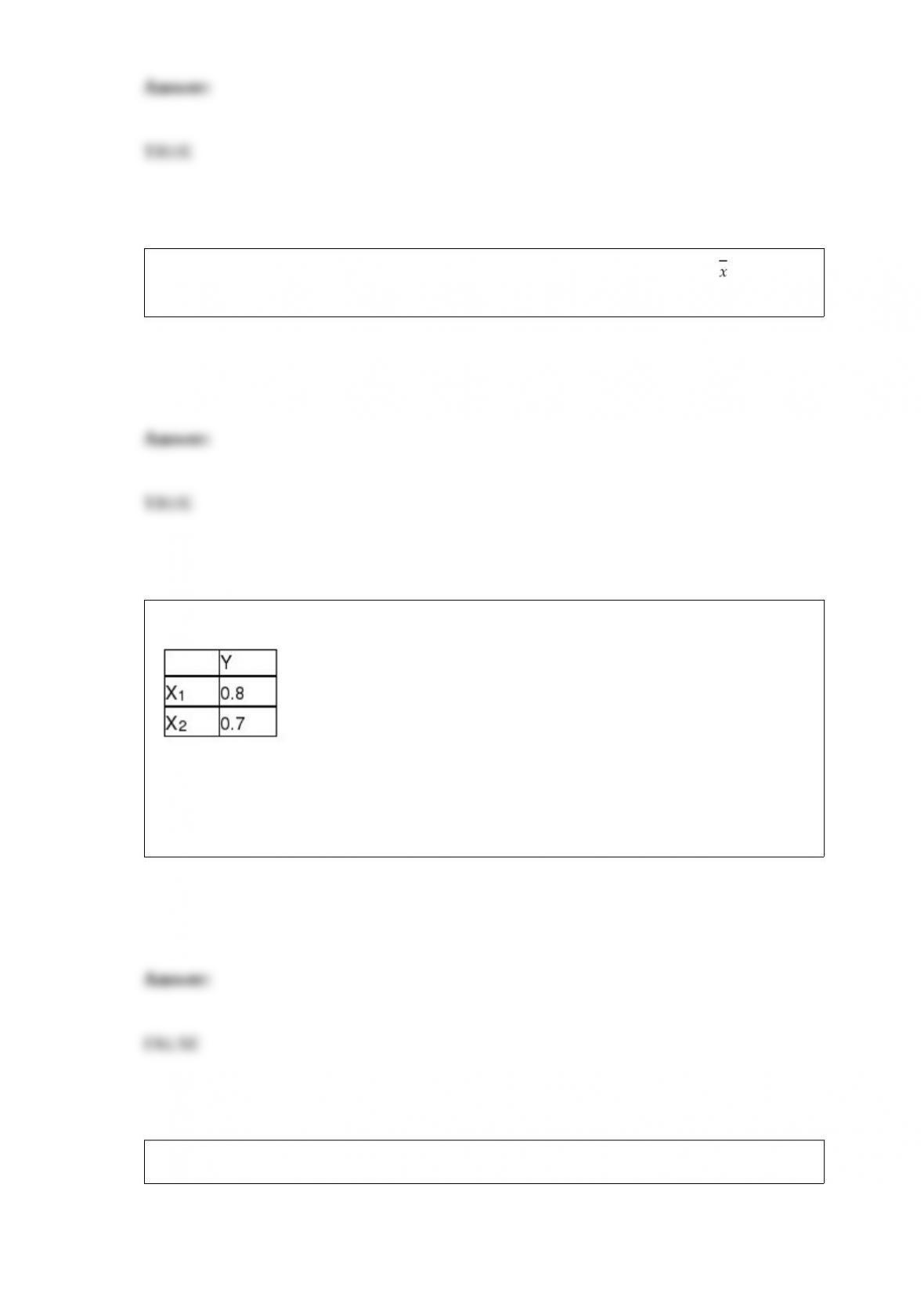
Based on the correlations below:
we could say that x1 accounts for 64 percent of the variation in y and x2 accounts for 49
percent of the variation in y. So if both xs are included in a multiple regression model,
then the resulting R-square = 1.13.
Choosing an alpha of 0.01 will cause beta to equal 0.99.

If a decision maker is concerned that the chance of making a Type II error is too large,
one option that will help reduce the risk is to reduce the significance level.
Managers use contingency analysis to determine whether two categorical variables are
independent of each other.
Stock analysts have recently stated in a meeting on Wall Street that over the past 50
years there have been periods of high market prices followed by periods of lower prices
but over time prices have moved upwards. Given their statement, stock prices most
likely exhibit only trend and cyclical components.
The Wilcoxon Matched-Pairs Signed rank test is an alternative to the paired sample
t-test when we are unwilling to assume that the populations are normally distributed.
A parameter is the boundary on the population of interest.
Confidence intervals constructed with small samples tend to have greater margins of
error than those constructed from larger samples, all else being constant.
If a population is normally distributed, then the sampling distribution for the sample
mean will always be normally distributed regardless of the sample size.
If a decision maker desires a small margin of error and a high level of confidence, it is
certain that the required sample size will be quite large.
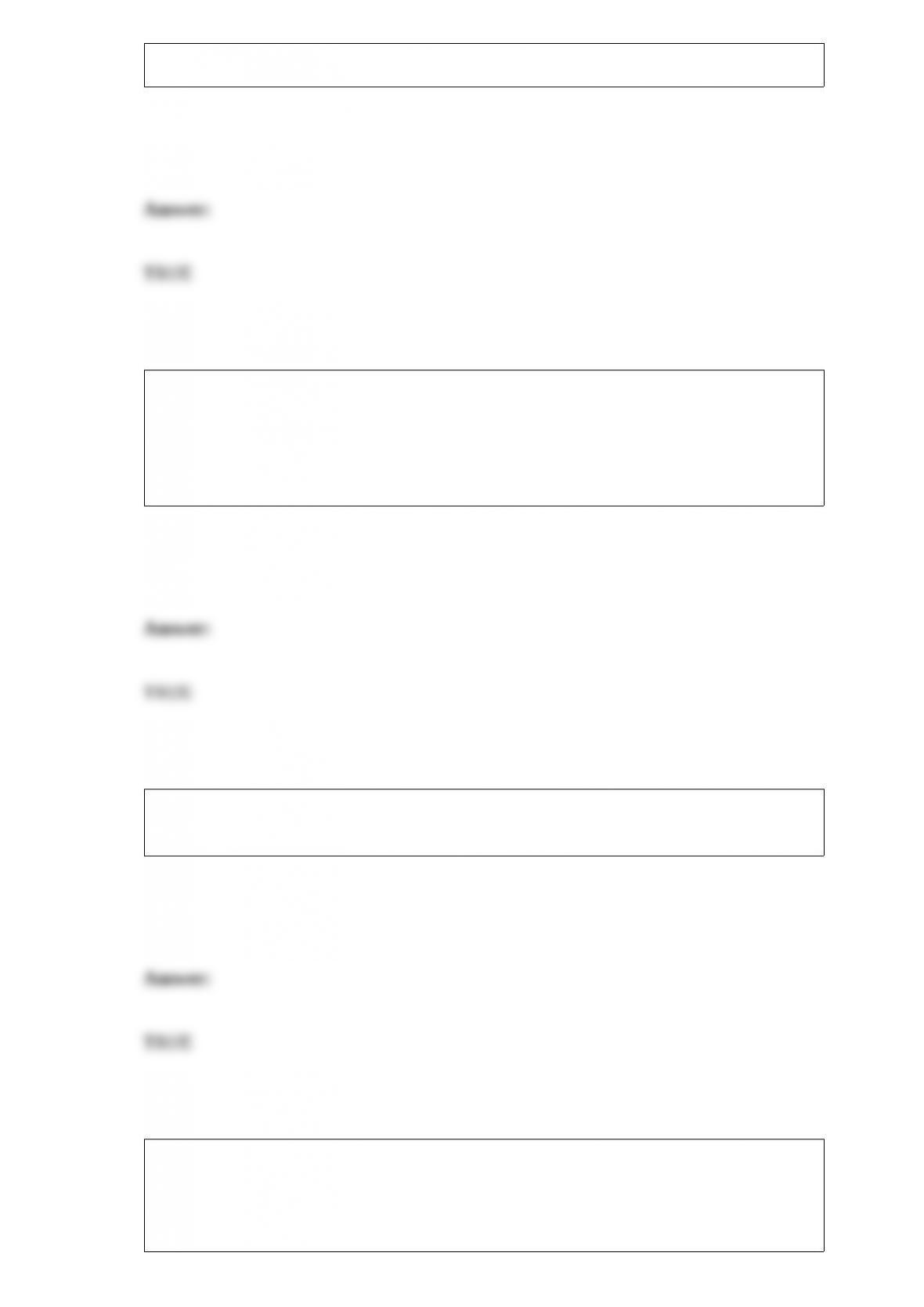
There is interest at the American Savings and Loan as to whether there is a difference
between average daily balances in checking accounts that are joint accounts (two or
more members per account) versus single accounts (one member per account). To test
this, a random sample of checking accounts was selected with the following results:
Based upon these data, assuming that the populations are normally distributed with
equal variances, the test statistic for testing whether the two populations have equal
means is approximately -1.49.
An experiment is a process that generates data as its outcome.
A major package delivery company claims that at least 95 percent of the packages it
delivers reach the destination on time. As part of the evidence in a lawsuit against the
package company, a random sample of n = 200 packages was selected. A total of 188 of
these packages were delivered on time. Using a significance level of .05, the test
statistic for this test is approximately z = -0.65.
One of the assumptions associated with the Wilcoxon Matched-Pairs Signed Rank test
is that the distribution of the population differences is symmetric about their median.
The Sergio Lumber Company manufactures plywood. One step in the process is the one
where the veneer is dried by passing through a huge dryer (similar to an oven) where
much of the moisture in the veneer is extracted. At the end of this step, samples of
veneer are tested for moisture content. It is believed that pine veneer will be less moist
on average than will fir veneer. The hypothesis test that will be conducted using an
alpha = 0.05 level will be a two-tailed test.
When surveyed, a sample of 1,250 patients at a regional hospital provided interviewers
with the following summary statistics pertaining to the hospital charges:
Minimum = $278.00 Q1 = $1,245 Q2 = $3,567 Q3= $4,702.
Based on these data, if you were to construct a box and whisker plot, the value
corresponding to the right-hand edge of the box would be $4,702.
If the point estimate in a paired difference estimation example does not fall in the
resulting confidence interval, the decision maker can conclude that the two populations
likely have different means.
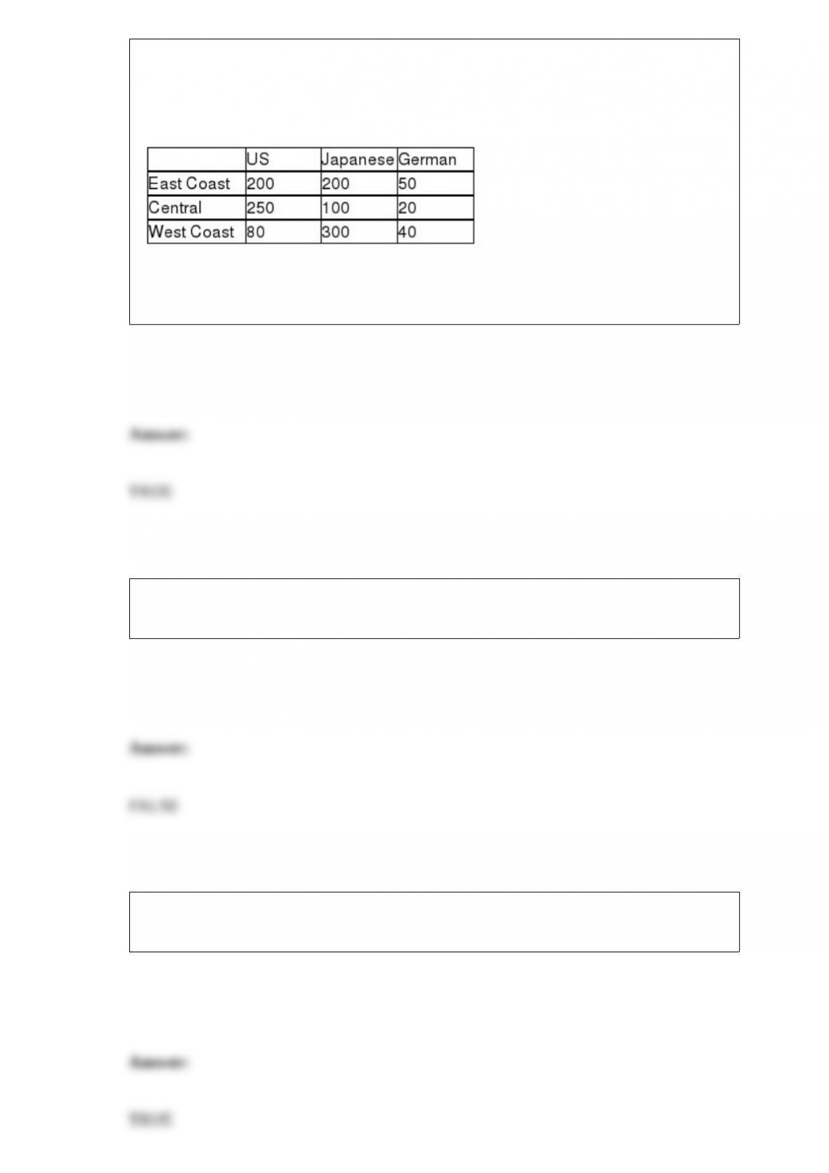
A study was recently done in the United States in which car owners were asked to
indicate whether their most recent car purchase was a U.S. car, a German car, or a
Japanese car. The people in the survey were divided by geographic region in the United
States. The following data were recorded.
Given this situation, to test whether the car origin is independent of the geographical
location of the buyer, the sum of the expected cell frequencies will equal 1,240.
If the probability of a Type I error is set at 0.05, then the probability of a Type II error
will be 0.95.
When using the Histogram tool in Excel to construct a frequency distribution and
histogram, the bins represent the upper class limits.
When the Histogram tool in Excel is used to construct a frequency distribution and
histogram, the default histogram is in the proper format and will require only that you
add appropriate labels.
Sampling error can be eliminated if the sampling is done properly.
A sample of n observations is taken from a normally distributed population to estimate
the population variance. The degrees of freedom for the chi-square distribution are n-2.
While virtually all time series exhibit a random component, not all time series exhibit
other components.

If we are interested in performing a one-tailed, upper-tail hypothesis test about a
population variance where the level of significance is .05 and the sample size is n = 20,
the critical chi-square value to be used is 30.1435.
A decision maker is considering constructing a multiple regression model with two
independent variables. The correlation between x1 and y is 0.70, and the correlation
between variable x2 and y is 0.50. Based on this, the regression model containing both
independent variables will explain 74 percent of the variation in the dependent variable.
A product that is produced at Ramsey Manufacturing goes through three steps to be
built. At step one, the components are assembled by technicians. At step two, the
product is sanded, and at step three the product is painted. The product can become
defective if any of these three steps is performed incorrectly. The three steps are done
by different people in different locations. We let D1 = defect introduced at step 1, D2 =
defect introduced at step 2, and D3 = defect introduced at step three. Based on this
situation these three events would be considered to be mutually exclusive.
Unlike the case of goodness-of-fit testing, with contingency analysis there is no
restriction on the minimum size for an expected cell frequency.
When the intercept in a regression equation is deemed not significantly different from 0,
then in making predictions for y, 0.0 should be used as the value of the intercept rather
than the estimated intercept value.
An Internet service provider is interested in estimating the proportion of homes in a
particular community that have computers but do not already have Internet access. To
do this, the company has selected a random sample of n = 200 homes and made calls. A
total of 188 homes responded to the survey question with 38 saying that they had a
computer with no Internet access. The 95 percent confidence interval estimate for the
true population proportion is approximately 0.1447 – 0.2595.

It is possible for the standard error of the estimate to actually increase if variables are
added to the model that do not aid in explaining the variation in the dependent variable.
A study recently conducted by a marketing firm analyzed three different advertising
designs and four different income levels of potential customers. At each combination of
factor A and factor B, 5 customers are observed and the number of products produced
are recorded. The degrees of freedom for the MSE in this two-factor ANOVA design is
48.
A recent study of students at the university contained data on year in school and student
age. An appropriate tool for analyzing the relationship between these two variables
would be a joint frequency distribution.

If cars arrive to a service center randomly and independently at a rate of 5 per hour on
average, what is the probability that exactly 5 cars will arrive during a given hour?
A) 0.1755
B) 0.6160
C) 0.1277
D) Essentially zero
The number of customers who enter a bank is thought to be Poisson distributed with a
mean equal to 10 per hour. What are the chances that 2 or 3 customers will arrive in a
15-minute period?
A) 0.0099
B) 0.4703
C) 0.0427
D) 0.0053

A random variable, x, has a normal distribution with μ = 13.6 and σ = 2.90. Determine a
value, x0, so that P(x > x0) = 0.05.
A) 14.46
B) 15.33
C) 18.37
D) 12.45
Which of the following will be helpful if the decision maker wishes to reduce the
chance of making a Type II error?
A) Increase the level of significance at which the hypothesis test is conducted.
B) Increase the sample size.
C) Both A and B will work.
D) Neither A nor B will be effective.
Given a binomial distribution with n = 8 and p = 0.40, obtain the probability that the
number of successes is within 2 standard deviations of the mean.
A) 0.6887
B) 0.7334
C) 0.8665
D) 0.9334
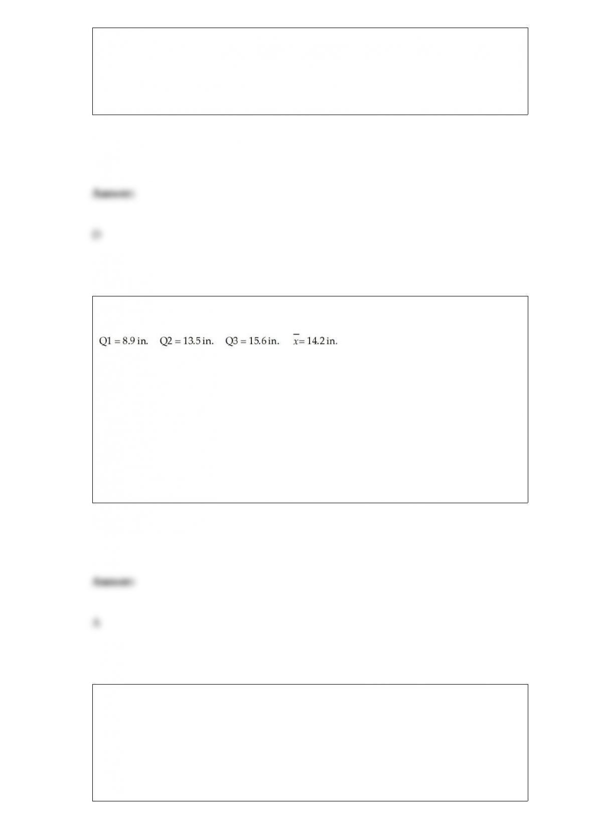
At a sawmill in Oregon, a process improvement team measured the diameters for a
sample of 1,500 logs. The following summary statistics were computed:
Given this information, the boundaries on the box in a box and whisker plot are:
A) 8.9 in and 15.6 in.
B) 13.5 in 1.5 (Q3-Q1).
C) 14.2 in 1.5 (Q3-Q1).
D) 8.9 in and 14.2 in.
In a multiple regression, the dependent variable is house value (in ‘000$) and one of the
independent variables is a dummy variable, which is defined as 1 if a house has a
garage and 0 if not. The coefficient of the dummy variable is found to be 5.4 but the
t-test reveals that it is not significant at the 0.05 level. Which of the following is true?
A) A garage increases the house value by $5,400.

B) A garage increases the house value by $5,400, holding all other independent
variables constant.
C) The house value remains the same with or without a garage.
D) We need to include other dummy variables.
The degrees of freedom for the chi-square goodness-of-fit test are equal to ________,
where k is the number of categories.
A) k + 1
B) k – 1
C) k + 2
D) k – 2
Data was collected on the number of television sets in a household, and it was found
that the mean was 3.5 and the standard deviation was 0.75.
Based on these sample data, what is the standardized value corresponding to 5
televisions?
A) -2.00
B) 1.5

C) 2.00
D) 1.125
The number of weeds that remain living after a specific chemical has been applied
averages 1.3 per square yard and follows a Poisson distribution. Based on this, what is
the probability that a 1-square yard section will contain less than 4 weeds?
A) 0.0324
B) 0.0998
C) Nearly 0.5000
D) 0.9569
A major cell phone service provider has determined that the number of minutes that its
customers use their phone per month is normally distributed with a mean equal to 445.5
minutes with a standard deviation equal to 177.8 minutes. The company is thinking of
changing its fee structure so that anyone who uses the phone less than 250 minutes
during a given month will pay a reduced monthly fee. Based on the available
information, what percentage of current customers would be eligible for the reduced
fee?
A) About 36.4 percent
B) Approximately 52 percent
C) About 86.6 percent
D) About 13.6 percent
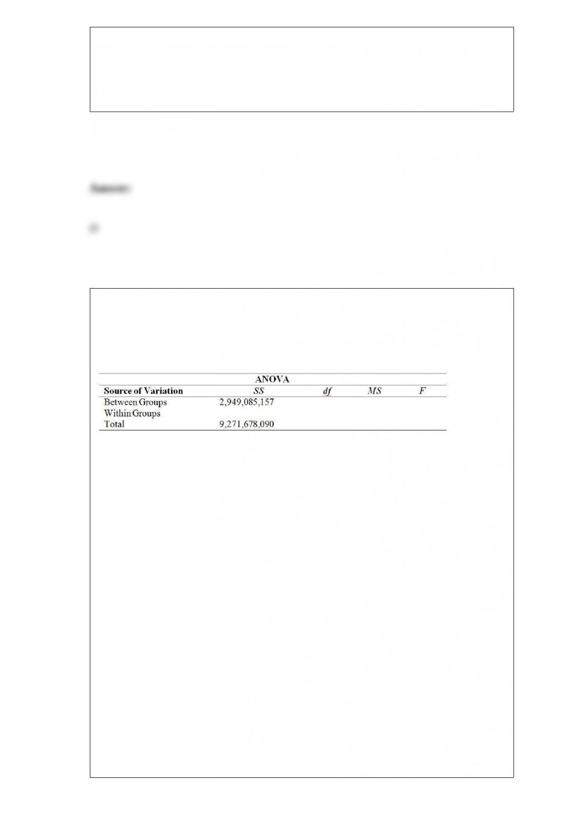
A start-up cell phone applications company is interested in determining whether
house-hold incomes are different for subscribers to three different service providers. A
random sample of 25 subscribers to each of the three service providers was taken, and
the annual household income for each subscriber was recorded. The partially completed
ANOVA table for the analysis is shown here:
Based on the sample results, can the start-up firm conclude that there is a difference in
household incomes for subscribers to the three service providers? You may assume
normal distributions and equal variances. Conduct your test at the alpha= 0.10 level of
significance. Be sure to state a critical F-statistic, a decision rule, and a conclusion.
A) H0: 1 = 2 = 3HA: Not all populations have the same mean
F = MSB/MSW = 1,474,542,579/87,813,791 = 16.79
Because the F test statistic = 16.79 > Fα = 2.3778, we do reject the null hypothesis
based on these sample data.
B) H0: 1 = 2 = 3HA : Not all populations have the same mean
F = MSB/MSW = 87,813,791 /1,474,542,579= 0.060
Because the F test statistic = 0.060 < Fα = 2.3778, we do not reject the null hypothesis
based on these sample data.
C) H0 : 1 = 2 = 3HA : Not all populations have the same mean

F = SSW/MSW = 6,322,592,933/87,813,791 = 72
Because the F test statistic = 72 > Fα = 2.3778, we do reject the null hypothesis based
on these sample data.
D) H0 : 1 = 2 = 3HA : Not all populations have the same mean
F = SSW/MSW = 6,322,592,933/1,474,542,579= 4.28
Because the F test statistic = 4.28 > Fα = 2.3778, we do reject the null hypothesis based
on these sample data
For the following z-test statistic, compute the p-value assuming that the hypothesis test
is a one-tailed test: z = 1.34.
A) 0.0606
B) 0.0815
C) 0.0124
D) 0.0901
The results of a census of 2,500 employees of a mid-sized company with 401(k)
retirement accounts are as follows:
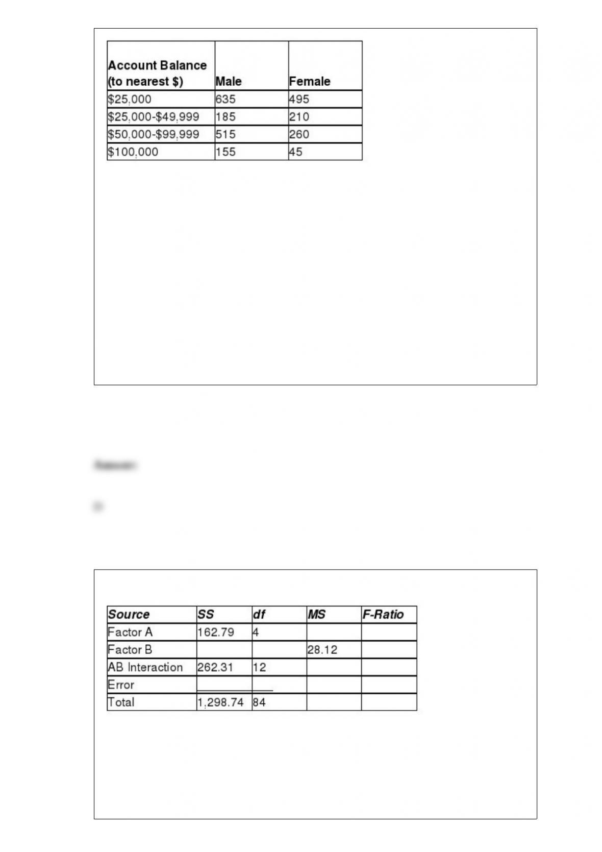
Suppose researchers are going to sample employees from the company for further
study.
Based on the relative frequency assessment method, what is the probability that a
randomly selected employee will be a female?
A) 0.1580
B) 0.1040
C) 0.6160
D) 0.4040
Examine the following two-factor analysis of variance table:
Does the ANOVA table indicate that the levels of factor B have equal means? Use a
significance level of 0.05.
A) Fail to reject H0. Conclude that there is not sufficient evidence to indicate that at
least two levels of Factor B have different mean responses.

B) Reject H0. Conclude that there is sufficient evidence to indicate that at least two
levels of Factor B have different mean responses.
C) Fail to reject H0. Conclude that there is sufficient evidence to indicate that at least
two levels of Factor B have different mean responses.
D) Reject H0. Conclude that there is not sufficient evidence to indicate that at least two
levels of Factor B have different mean responses.
Which of the following is not a required step in finding beta?
A) Assuming a true value of the population parameter where the null is false
B) Finding the critical value based on the null hypothesis
C) Converting the critical value from the standard normal distribution to the units of the
data
D) Finding the power of the test
In analyzing the relationship between two variables, a scatter plot can be used to detect
which of the following?
A) A positive linear relationship

B) A curvilinear relationship
C) A negative linear relationship
D) All of the above
The transportation manager for the State of New Jersey has determined that the time
between arrivals at a toll booth on the state’s turnpike is exponentially distributed with λ
= 4 cars per minute. Based on this information, what is the probability that the time
between any two cars arriving will exceed 11 seconds?
A) Approximately 1.0
B) Approximately 0.48
C) About 0.52
D) About 0.75
Which of the following is not a characteristic of the normal distribution?
A) Symmetric
B) Mean = median = mode
C) Bell-shaped

D) Equal probabilities at all values of x
Joint frequency distributions are used to display:
A) the histograms of two variables analyzed simultaneously.
B) the number of occurrences at each of the possible joint occurrences of two variables.
C) the cumulative distribution of a variable with two possible outcomes.
D) the relative frequency of two variables.
In a standard normal distribution, the probability P(-1.00< z < 1.20) is the same as:
A) P(1< z < 1.20) – P(0 < z < 1.00).
B) P(1< z < 1.20) – 2*P(0 < z < 1.00).
C) 2 P(1< z < 1.20) – P(0 < z <1.00).∗
D) P(1 < z < 1.20) + 2 P(0 < z <1.00). ∗

A consulting report that was recently submitted to a company indicated that a
hypothesis test for a single population variance was conducted. The report indicated
that the test statistic was 34.79, the hypothesized variance was 345 and the sample
variance 600. However, the report did not indicate what the sample size was. What was
it?
A) n = 100
B) Approximately n = 18
C) Approximately 21
D) Can’t be determined without knowing what alpha is.
Under what conditions can the t-distribution be correctly employed to test the difference
between two population means?
A) When the samples from the two populations are small and the population variances
are unknown
B) When the two populations of interest are assumed to be normally distributed
C) When the population variances are assumed to be equal
D) All of the above
A small city is considering breaking away from the county school system and starting
its own city school system. City leaders believe that more than 60 percent of residents
support the idea. A poll of n = 215 residents is taken and 134 people say they support
starting a city school district. Using a 0.10 level of significance, conduct a hypothesis
test to determine whether this poll supports the belief of city leaders.

The managers at Harris Pizza in Boston have tracked the tips received by their drivers
along with the total bill to the customer. An appropriate graph for analyzing the
relationship between these two variables is:
A) a scatter diagram.
B) a line chart.
C) a histogram.
D) a pie chart.
How can the degrees of freedom be found in a contingency table with cross-classified
data?
A) When df are equal to rows minus columns
B) When df are equal to rows multiplied by columns
C) When df are equal to rows minus 1 multiplied by columns minus 1
D) Total number of cell minus 1
A study was recently conducted at a major university to estimate the difference in the
proportion of business school graduates who go on to graduate school within five years
after graduation and the proportion of non-business school graduates who attend
graduate school. A random sample of 400 business school graduates showed that 75 had

gone to graduate school while in a random sample of 500 non-business graduates, 137
had gone on to graduate school. Based on a 95 percent confidence level, what is the
upper limit of the confidence interval estimate?
A) 0.2340
B) 0.1034
C) -0.031
D) -0.018
Both p-charts and c-charts are designed for use when the data we are working with are
referred to as attribute data.
A hotel chain has four hotels in Oregon. The general manager is interested in
determining whether the mean length of stay is the same or different for the four hotels.
She selects a random sample of n = 20 guests at each hotel and determines the number
of nights they stayed. Assuming that she plans to test this using an alpha level equal to
0.05, which of the following is the correct critical value?
A) F = 3.04
B) F = 2.76
C) t = 1.9917
D) F = 2.56
When the park ranger at Yellowstone National Park reports the average length of time
that visitors spend in the park, he is using:
A) graphical tools.
B) numerical measures.
C) statistical charts.
D) histograms or bar charts.
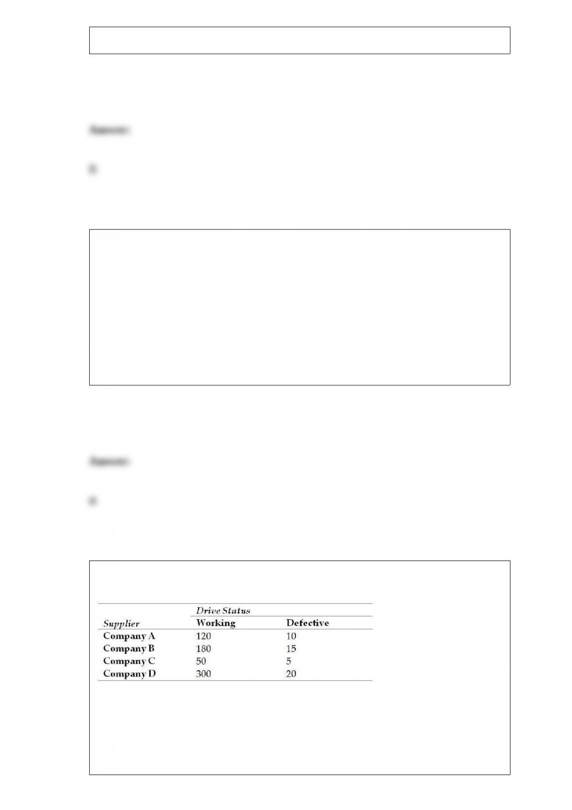
Suppose a quality manager for Dell Computers has collected the following data on the
quality status of disk drives by supplier. She inspected a total of 700 disk drives.
What is the probability of a defective disk drive being received by the computer
company?
A) 0.07

B) 0.28
C) 0.021
D) 0.76
Suppose a study of 196 randomly sampled privately insured adults with incomes over
200% of the current poverty level is to be used to measure out-of-pocket medical
expenses for prescription drugs for this income class. The sample data are in the file
Drug Expenses.
Based on the sample data, construct a 95% confidence interval estimate for the mean
annual out-of-pocket expenditures on prescription drugs for this income class. Interpret
this interval.
A) (162.08, 172.96)
B) (163.50, 171.54)
C) (164.19, 170.85)
D) (161.97, 173.07)
The following regression output was generated based on a sample of utility customers.
The dependent variable was the dollar amount of the monthly bill and the independent
variable was the size of the house in square feet.
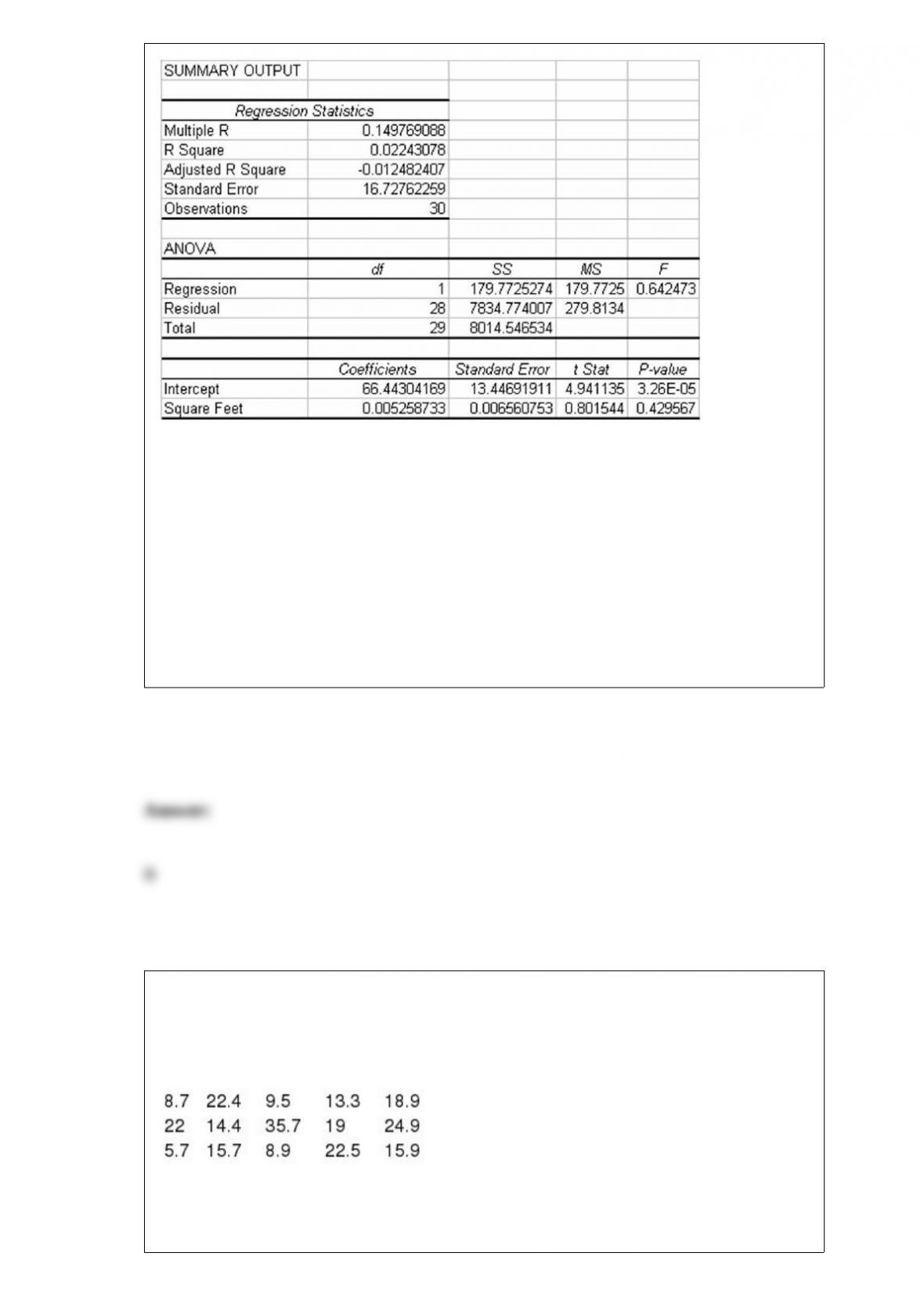
Based on this regression output, what is the 95 percent confidence interval estimate for
the population regression slope coefficient?
A) Approximately -0.0003 —– +0.0103
B) About -0.0082 —– +0.0188
C) Approximately -32.76 —– +32.79
D) None of the above
One of the major oil products companies conducted a study recently to estimate the
mean gallons of gasoline purchased by customers per visit to a gasoline station. To do
this, a random sample of customers was selected with the following data being recorded
that show the gallons of gasoline purchased.
Based on these sample data, construct and interpret a 95 percent confidence interval
estimate for the population mean.
Suppose a population is normally distributed with a mean 100 and a standard deviation
of 15. When a sample of size n = 36 is collected a sampling distribution is created.
Explain which is larger: the probability of a value randomly selected from the
population being larger than 120, or the probability of a sample mean being larger than
120.
When estimating the difference between two population means, when should the
normal distribution be used and when should the t-distribution be used?

Open the data file provided with the text called Computer Use. Indicate the level of data
measurement for each variable in the data set.
A major U.S. oil company has developed two blends of gasoline. Managers are
interested in determining whether a difference in mean gasoline mileage will be
obtained from using the two blends. As part of their study, they have decided to run a
test using the Chevrolet Impala automobile with automatic transmissions. They selected
a random sample of 100 Impalas using Blend 1 and another 100 Impalas using Blend 2.
Each car was first emptied of all the gasoline in its tank and then filled with the
designated blend of the new gasoline. The car was then driven 200 miles on a specified
route involving both city and highway roads. The cars were then filled and the actual
miles per gallon were recorded. The following summary data were recorded:
Blend 1 Blend 2
Sample Size 100 100
Sample Mean 23.4 mpg 25.7 mpg
Sample St. Dev. 4.0 mpg 4.2 mpg
Based on the sample data, using a 0.05 level of significance, what conclusion should the
company reach about whether the population mean mpg is the same or different for the
two blends? Use the p-value approach to test the null hypothesis.
Explain what information can be conveyed by a frequency histogram.
The binomial distribution is frequently used to help companies decide whether to accept
or reject a shipment based on the results of a random sample of items from the
shipment. For instance, suppose a contract calls for, at most, 10 percent of the items in a
shipment to be red. To check this without looking at every item in the large shipment, a
sample of n = 10 items is selected. If 1 or fewer are red, the shipment is accepted;
otherwise it is rejected. Using probability, determine whether this is a “good” sampling
plan. (Assume that a bad shipment is one that has 20 percent reds.)
The Swanson Auto Body business repaints cars that have been in an accident or which
are in need of a new paint job. Its quality standards call for an average of 1.2 paint
defects per door panel. Explain why there is a difference between the probability of
finding exactly 1 defect when 1 door panel is inspected and finding exactly 2 defects
when 2 doors are inspected.
The Gordon Beverage Company bottles soft drinks using an automatic filling machine.
When the process is running properly, the mean fill is 12 ounces per can. The machine
has a known standard deviation of 0.20 ounces. Each day, the company selects a
random sample of 36 cans and measures the volume in each can. They then test to
determine whether the filling process is working properly. The test is conducted using a
0.05 significance level. Using the test statistic approach, what conclusion should the
company reach if the sample mean is 12.02 ounces? What type of statistical error may
have been committed?
Explain why, in performing a goodness-of-fit test, it is sometimes necessary to combine
categories.
What is the underlying common element of all statistical sampling techniques?
The accountant for a large U.S. company is interested in finding the probability that an
account will have an incorrect balance due to being overstated or being understated. To
find this probability, which probability rule is she likely to use?
The fares received by taxi drivers working for the City Taxi line are normally
distributed with a mean of $12.50 and a standard deviation of $3.25. Suppose a driver
has four consecutive fares that are less than $6.00. What is the probability of this
happening?
In a recent audit report, an accounting firm stated that the mean sale per customer for
the client was estimated to be between $14.50 and $28.50. Further, this was based on a
random sample of 100 customers and was computed using 95 percent confidence.
Provide a correct interpretation of this confidence interval estimate.
Discuss the two major types of descriptive statistics.
A maker of toothpaste is interested in testing whether the proportion of adults (over age
18) who use its toothpaste and have no cavities within a six-month period is any
different from the proportion of children (18 and under) who use the toothpaste and
have no cavities within a six-month period. To test this, it has selected a sample of
adults and a sample of children randomly from the population of those customers who
use their toothpaste. The following results were observed.
Adults Children
Sample size 100 200
Number with 0 cavities 83 165
Based on these sample data and using a significance level of 0.05, what conclusion
should be reached? Use the p-value approach to conduct the test.