True or False: Holding the sample size fixed, increasing the level of confidence in a
confidence interval will necessarily lead to a wider confidence interval.
TABLE 8-5
A sample of salary offers (in thousands of dollars) given to management majors is: 48,
51, 46, 52, 47, 48, 47, 50, 51, and 59. Using this data to obtain a 95% confidence
interval resulted in an interval from 47.19 to 52.61.
True or False: Referring to Table 8-5, a 99% confidence interval for the mean of the
population from the same sample would be wider than 47.19 to 52.61.
True or False: The t distribution allows the calculation of confidence intervals for
means when the actual standard deviation is not known.
True or False: The Central Limit Theorem ensures that the sampling distribution of the
sample mean approaches a normal distribution as the sample size increases.
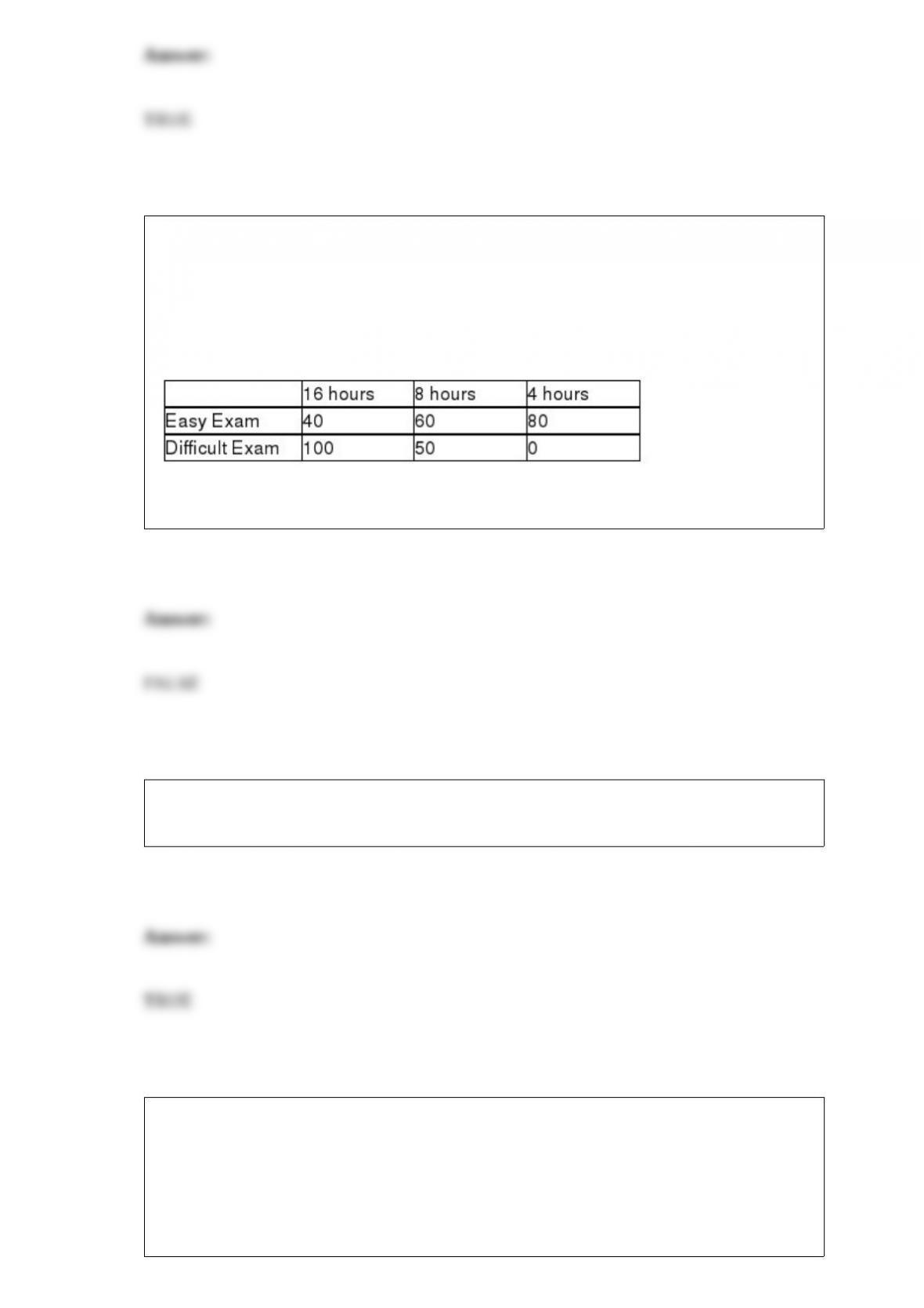
True or False: TABLE 19-6
A student wanted to find out the optimal strategy to study for a Business Statistics
exam. He constructed the following payoff table based on the mean amount of time he
needed to study every week for the course and the degree of difficulty of the exam.
From the information that he gathered from students who had taken the course, he
concluded that there was a 40% probability that the exam would be easy.
Referring to Table 19-6, the optimal strategy using the maximin criterion is to study 16
hours per week on average for the exam.
True or False: An unbiased estimator will have a value, on average across samples,
equal to the population parameter value.
TABLE 8-9
A university wanted to find out the percentage of students who felt comfortable
reporting cheating by their fellow students. A survey of 2,800 students was conducted
and the students were asked if they felt comfortable reporting cheating by their fellow
students. The results were 1,344 answered “Yes” and 1,456 answered “No.”
True or False: Referring to Table 8-9, it is possible that the 99% confidence interval
calculated from the data will not contain the proportion of the student population who
feel comfortable reporting cheating by their fellow students.
True or False: The line drawn within the box of the boxplot always represents the
arithmetic mean.
TABLE 14-15
The superintendent of a school district wanted to predict the
percentage of students passing a sixth-grade proficiency test. She
obtained the data on percentage of students passing the proficiency
test (% Passing), mean teacher salary in thousands of dollars
(Salaries), and instructional spending per pupil in thousands of dollars
(Spending) of 47 schools in the state.
Following is the multiple regression output with Y = % Passing as the
dependent variable, X1 = Salaries and X2 = Spending:

True or False: Referring to Table 14-15, you can conclude that
instructional spending per pupil has no impact on the mean
percentage of students passing the proficiency test, taking into
account the e.ect of mean teacher salary, at a 5% level of
significance using the confidence interval estimate for β2.
True or False: As a general rule, one can use the normal distribution to approximate a
binomial distribution whenever nand n( – 1) are at least 5.

True or False: Using different frames to generate data can lead to totally different
conclusions.
True or False: Sampling error becomes an ethical issue if the findings are purposely
presented without reference to sample size and margin of error so that the sponsor can
promote a viewpoint that might otherwise be truly insignificant.
TABLE 8-9
A university wanted to find out the percentage of students who felt comfortable
reporting cheating by their fellow students. A survey of 2,800 students was conducted
and the students were asked if they felt comfortable reporting cheating by their fellow
students. The results were 1,344 answered “Yes” and 1,456 answered “No.”
True or False: Referring to Table 8-9, we are 99% confident that the total number of the
student population who feel comfortable reporting cheating by their fellow students is
between 0.4557 and 0.5043.
True or False: TABLE 17-5
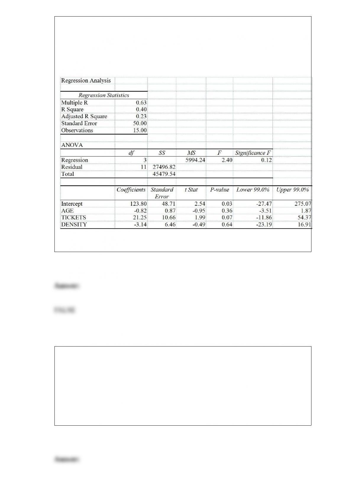
You worked as an intern at We Always Win Car Insurance Company last summer. You
notice that individual car insurance premiums depend very much on the age of the
individual, the number of traffic tickets received by the individual, and the population
density of the city in which the individual lives. You performed a regression analysis in
EXCEL and obtained the following information:
Referring to Table 17-5, the multiple regression model is significant at a 10% level of
significance.
The director of admissions at a state college is interested in seeing if admissions status
(admitted, waiting list, denied admission) at his college is related to the type of
community (urban, rural, suburban) in which an applicant resides. Which of the
following tests will be the most appropriate?
A) χ2 test for independence
B) Two-way ANOVA F test for the type of community effect
C) Two-way ANOVA F test for interaction effect
D) McNemar test
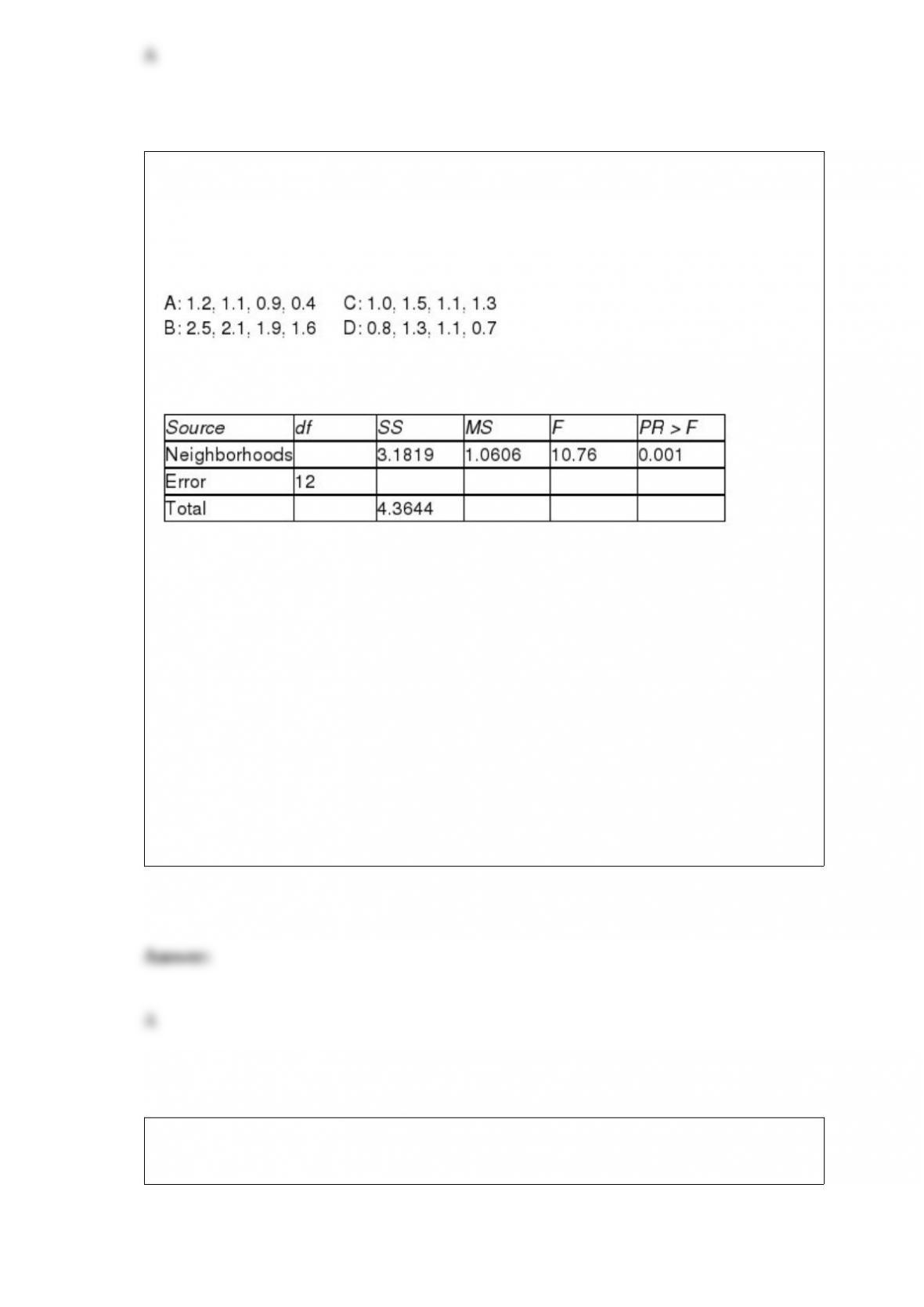
TABLE 11-2
A realtor wants to compare the mean sales-to-appraisal ratios of residential properties
sold in four neighborhoods (A, B, C, and D). Four properties are randomly selected
from each neighborhood and the ratios recorded for each, as shown below.
Interpret the results of the analysis summarized in the following table:
Referring to Table 11-2,
A) at the 0.05 level of significance, the mean ratios for the 4 neighborhoods are not all
the same.
B) at the 0.01 level of significance, the mean ratios for the 4 neighborhoods are all the
same.
C) at the 0.10 level of significance, the mean ratios for the 4 neighborhoods are not
significantly different.
D) at the 0.05 level of significance, the mean ratios for the 4 neighborhoods are not
significantly different from 0.
True of False: To determine the width of class interval, divide the number of class
groups by the range of the data.
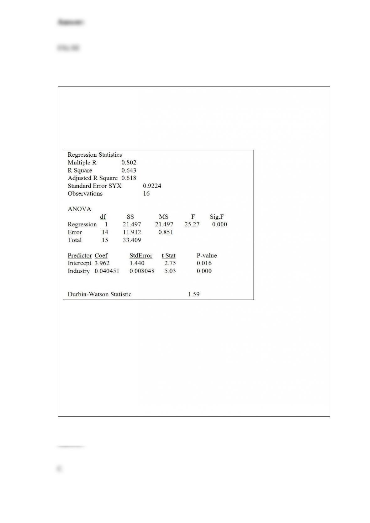
TABLE 13-5
The managing partner of an advertising agency believes that his company’s sales are
related to the industry sales. He uses Microsoft Excel to analyze the last 4 years of
quarterly data (i.e., n = 16) with the following results:
Referring to Table 13-5, the partner wants to test for autocorrelation using the
Durbin-Watson statistic. Using a level of significance of 0.05, the decision he should
make is
A) there is evidence of autocorrelation.
B) the test is unable to make a definite conclusion.
C) there is no evidence of autocorrelation.
D) there is not enough information to perform the test.

In a simple linear regression problem, r and b1
A) may have opposite signs.
B) must have the same sign.
C) must have opposite signs.
D) are equal.
The classification of student major (accounting, economics, management, marketing,
other) is an example of
A) a categorical variable.
B) a discrete variable.
C) a continuous variable.
D) a table of random numbers.
Referring to Table 14-15, which of the following is the correct null
hypothesis to determine whether there is a significant relationship
between percentage of students passing the proficiency test and the
entire set of explanatory variables?
TABLE 14-15
The superintendent of a school district wanted to predict the

percentage of students passing a sixth-grade proficiency test. She
obtained the data on percentage of students passing the proficiency
test (% Passing), mean teacher salary in thousands of dollars
(Salaries), and instructional spending per pupil in thousands of dollars
(Spending) of 47 schools in the state.
Following is the multiple regression output with Y = % Passing as the
dependent variable, X1 = Salaries and X2 = Spending:
A) H0 : β0 = β1 = β2 = 0
B) H0 : β1 = β2 = 0
C) H0 : β0 = β1 = β2 ≠0
D) H0 : β1 = β2 ≠0
TABLE 16-9
Given below are EXCEL outputs for various estimated autoregressive models for a
company’s real operating revenues (in billions of dollars) from 1989 to 2012. From the
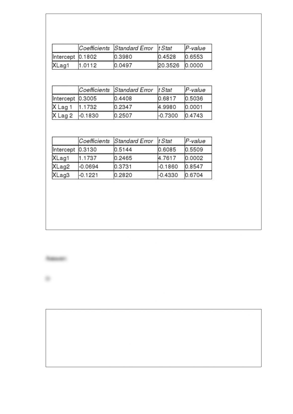
data, you also know that the real operating revenues for 2010, 2011, and 2012 are
11.7909, 11.7757 and 11.5537, respectively.
First-Order Autoregressive Model:
Second-Order Autoregressive Model:
Third-Order Autoregressive Model:
Referring to Table 16-9, if one decides to use the Third-Order Autoregressive model,
what will the predicted real operating revenue for the company be in 2015?
A) $11.59 billion
B) $11.68 billion
C) $11.84 billion
D) $12.47 billion
Referring to Table 14-5, what is the p-value for testing whether Capital has a positive
influence on corporate sales?
TABLE 14-5
A microeconomist wants to determine how corporate sales are influenced by capital and
wage spending by companies. She proceeds to randomly select 26 large corporations
and record information in millions of dollars. The Microsoft Excel output below shows
results of this multiple regression.
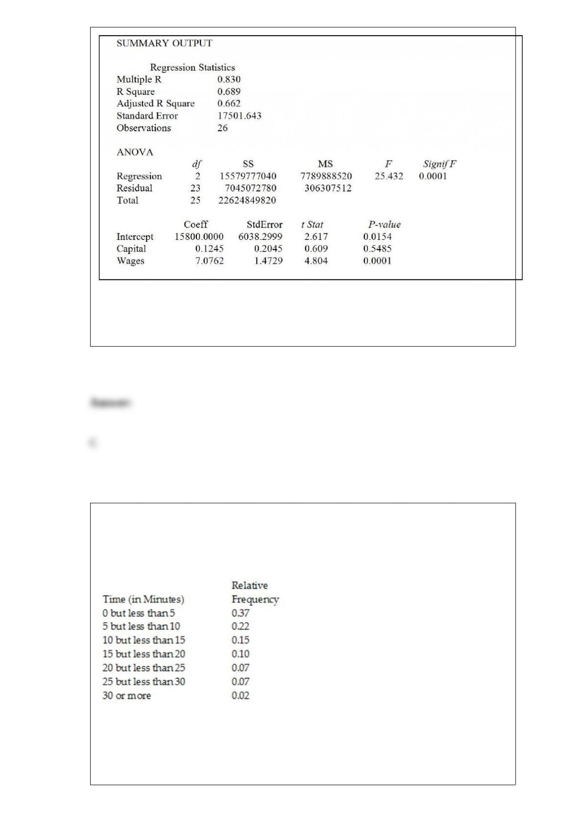
A) 0.025
B) 0.05
C) 0.2743
D) 0.5485
TABLE 2-5
The following are the duration in minutes of a sample of long-distance phone calls
made within the continental United States reported by one long-distance carrier.
Referring to Table 2-5, if 100 calls were sampled, ________ of them would have lasted
less than 15 minutes.
A) 26
B) 74
C) 10
D) None of the above.
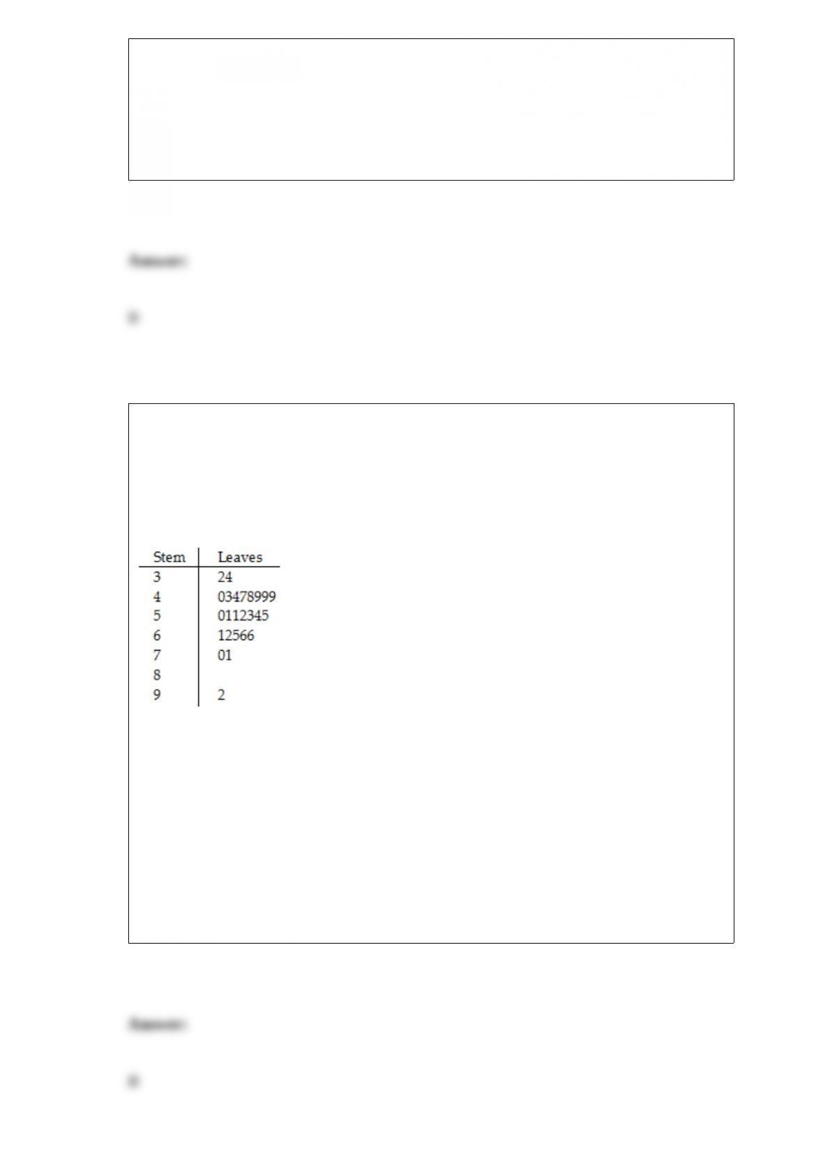
TABLE 2-4
A survey was conducted to determine how people rated the quality of programming
available on television. Respondents were asked to rate the overall quality from 0 (no
quality at all) to 100 (extremely good quality). The stem-and-leaf display of the data is
shown below.
Referring to Table 2-4, what percentage of the respondents rated overall television
quality with a rating of 80 or above?
A) 0
B) 4
C) 96
D) 100
The owner of a fish market has an assistant who has determined that the weights of
catfish are normally distributed, with a mean of 3.2 pounds and a standard deviation of
0.8 pound. If a sample of 16 fish is taken, what would the standard error of the mean
weight equal?
A) 0.003
B) 0.050
C) 0.200
D) 0.800
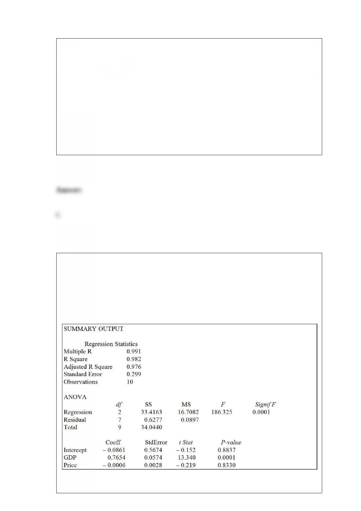
Referring to Table 14-3, to test whether gross domestic product has a positive impact on
consumption, the p-value is
TABLE 14-3
An economist is interested to see how consumption for an economy (in $ billions) is
influenced by gross domestic product ($ billions) and aggregate price (consumer price
index). The Microsoft Excel output of this regression is partially reproduced below.
A) 0.00005.
B) 0.0001.
C) 0.9999.
D) 0.99995.
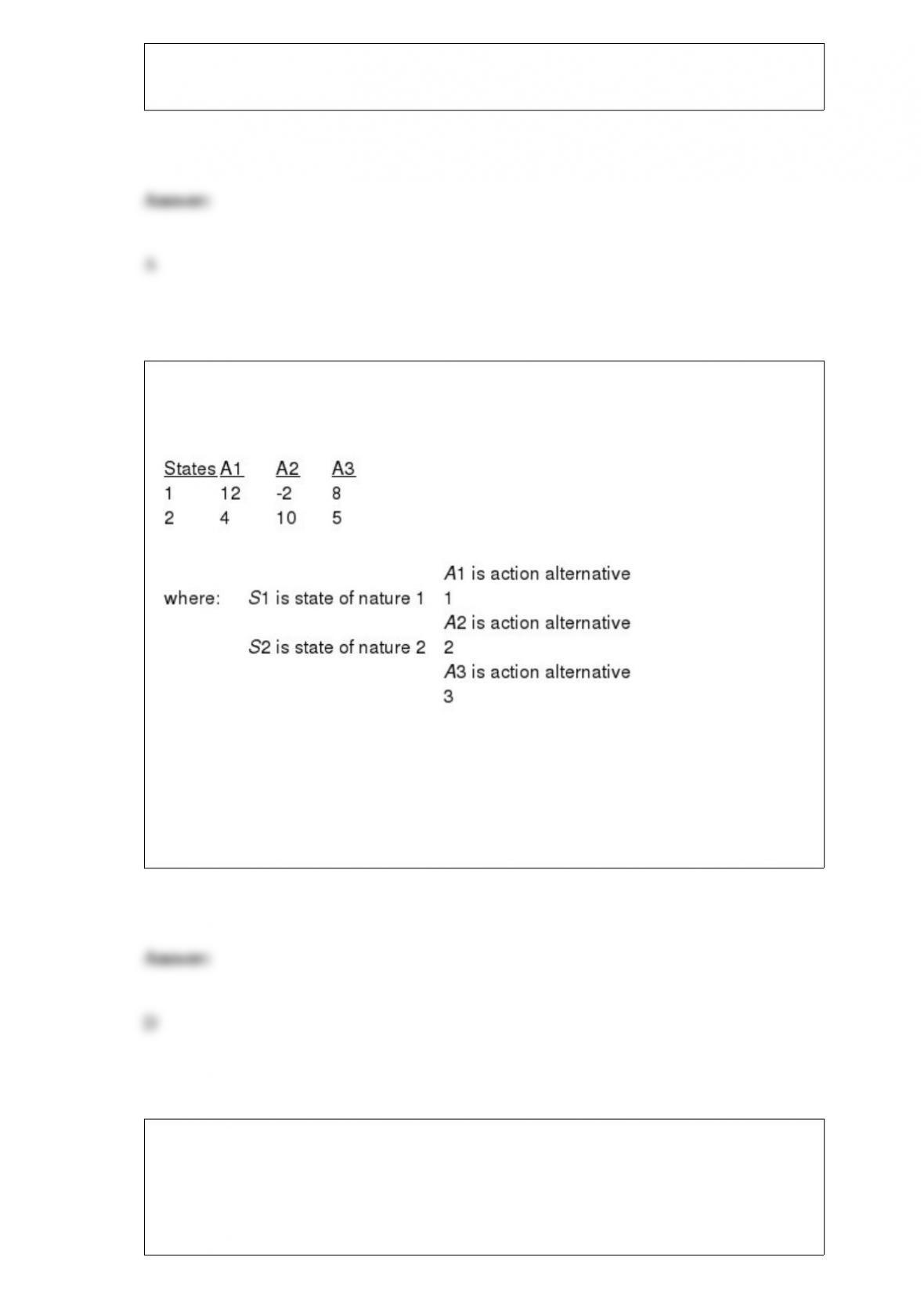
TABLE 19-1
The following payoff table shows profits associated with a set of 3 alternatives under 2
possible states of nature
Referring to Table 19-1, if the probability of S1 is 0.5, then the expected monetary value
(EMV) for A1 is
A) 3.
B) 4.
C) 6.5.
D) 8.
TABLE 8-1
The managers of a company are worried about the morale of their employees. In order
to determine if a problem in this area exists, they decide to evaluate the attitudes of their
employees with a standardized test. They select the Fortunato test of job satisfaction,
which has a known standard deviation of 24 points.
Referring to Table 8-1, due to financial limitations, the managers decide to take a
sample of 45 employees. This yields a mean score of 88.0 points. A 90% confidence
interval would go from ________ to ________.
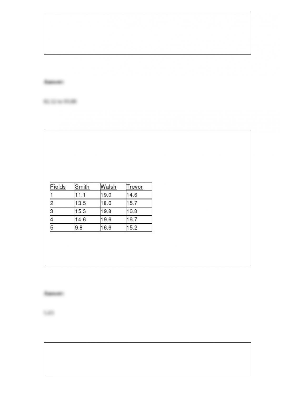
TABLE 11-10
An agronomist wants to compare the crop yield of 3 varieties of chickpea seeds. She
plants all 3 varieties of the seeds on each of 5 different patches of fields. She then
measures the crop yield in bushels per acre. Treating this as a randomized block design,
the results are presented in the table that follows.
Referring to Table 11-10, using an overall level of significance of 0.01, what is the
critical value of the Studentized range Q used in calculating the critical range for the
Tukey multiple comparison procedure?
TABLE 6-2
John has two jobs. For daytime work at a jewelry store he is paid $15,000 per month,
plus a commission. His monthly commission is normally distributed with a mean of
$10,000 and a standard deviation of $2,000. At night he works occasionally as a waiter,
for which his monthly income is normally distributed with a mean of $1,000 and a
standard deviation of $300. John’s income levels from these two sources are
independent of each other.
Referring to Table 6-2, the probability is 0.9 that John’s income as a waiter is less than
how much in a given month?
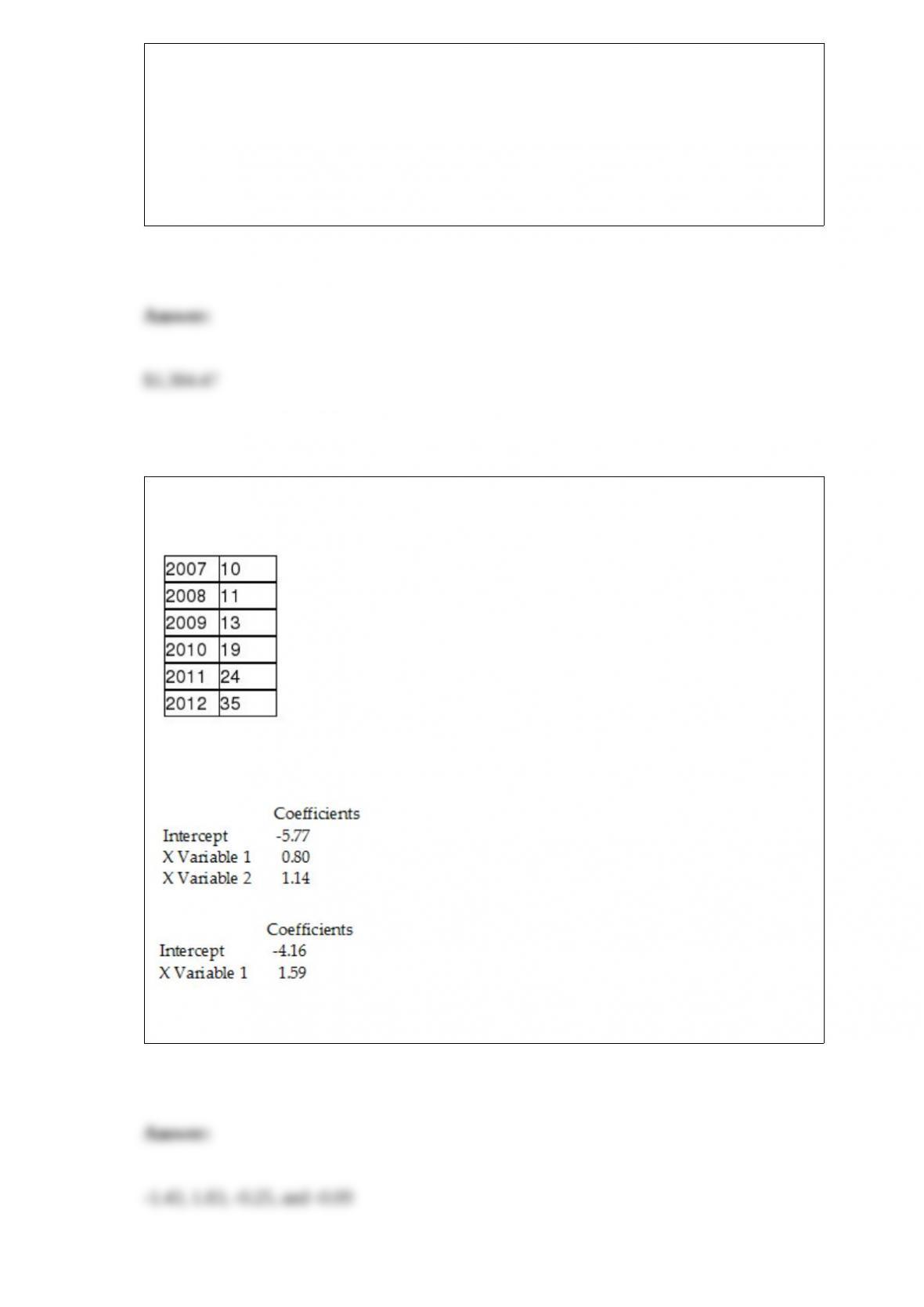
TABLE 16-10
Business closures in Laramie, Wyoming from 2007 to 2012 were:
Microsoft Excel was used to fit both first-order and second-order autoregressive
models, resulting in the following partial outputs:
SUMMARY OUTPUT – 2nd Order Model
SUMMARY OUTPUT – 1st Order Model
Referring to Table 16-10, the residuals for the second-order autoregressive model are
________, ________, ________, and ________.
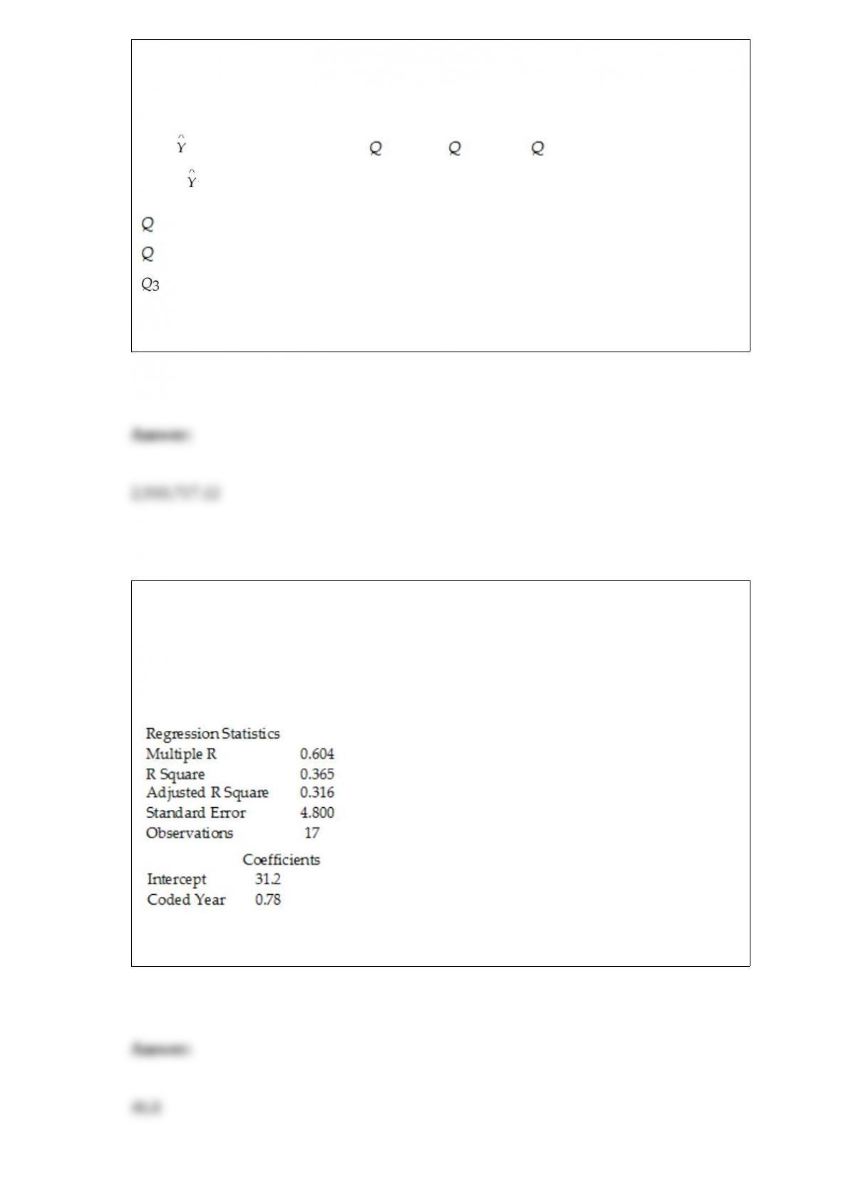
TABLE 16-12
A local store developed a multiplicative time-series model to forecast its revenues in
future quarters, using quarterly data on its revenues during the 5-year period from 2008
to 2012. The following is the resulting regression equation:
log10 = 6.102 + 0.012 X – 0.129 1 – 0.054 2 + 0.098 3
where is the estimated number of contracts in a quarter
X is the coded quarterly value with X = 0 in the first quarter of 2008
1 is a dummy variable equal to 1 in the first quarter of a year and 0 otherwise
2 is a dummy variable equal to 1 in the second quarter of a year and 0 otherwise
is a dummy variable equal to 1 in the third quarter of a year and 0 otherwise
Referring to Table 16-12, using the regression equation, what is the forecast for the
revenues in the third quarter of 2013?
TABLE 16-6
The president of a chain of department stores believes that her stores’ total sales have
been showing a linear trend since 1993. She uses Microsoft Excel to obtain the partial
output below. The dependent variable is sales (in millions of dollars), while the
independent variable is coded years, where 1993 is coded as 0, 1994 is coded as 1, etc.
SUMMARY OUTPUT
Referring to Table 16-6, the forecast for sales (in millions of dollars) in 2013 is
________.
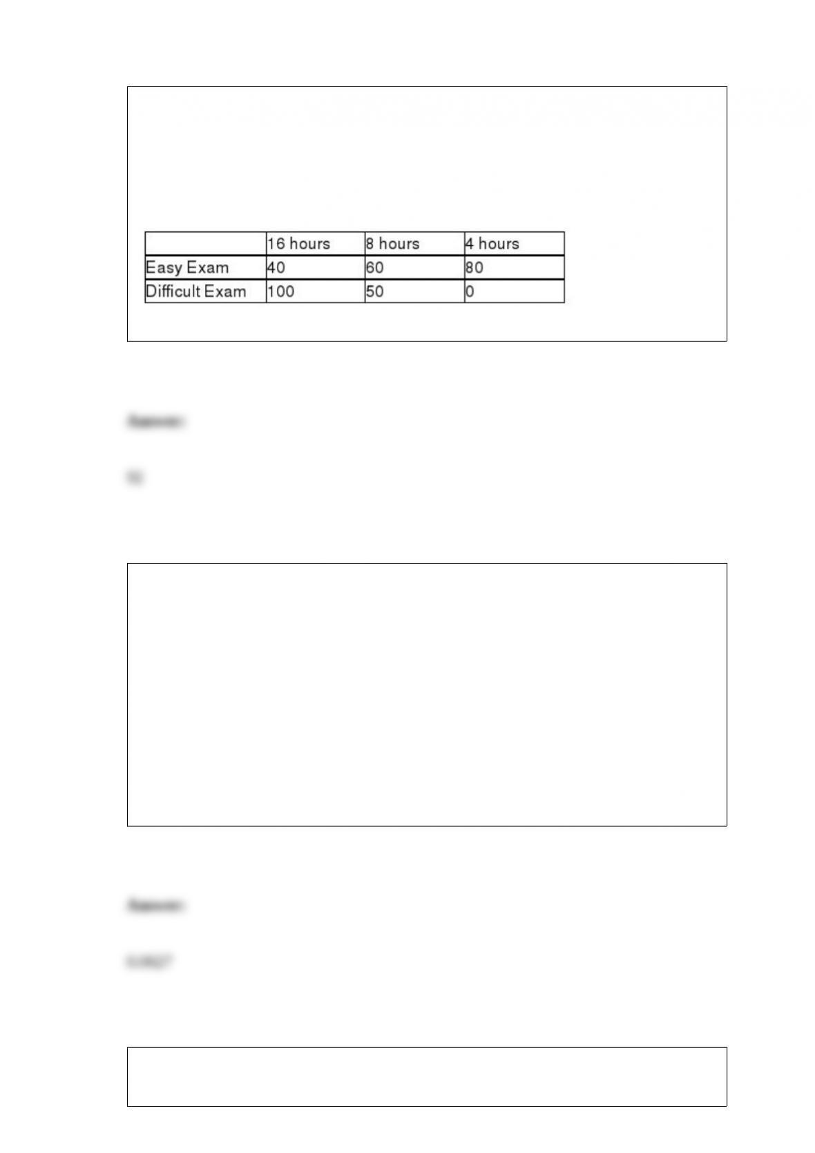
TABLE 19-6
A student wanted to find out the optimal strategy to study for a Business Statistics
exam. He constructed the following payoff table based on the mean amount of time he
needed to study every week for the course and the degree of difficulty of the exam.
From the information that he gathered from students who had taken the course, he
concluded that there was a 40% probability that the exam would be easy.
Referring to Table 19-6, what is the expected profit under certainty?
TABLE 9-9
The president of a university claimed that the entering class this year appeared to be
larger than the entering class from previous years but their mean SAT score is lower
than previous years. He took a sample of 20 of this year’s entering students and found
that their mean SAT score is 1,501 with a standard deviation of 53. The university’s
record indicates that the mean SAT score for entering students from previous years is
1,520. He wants to find out if his claim is supported by the evidence at a 5% level of
significance.
Referring to Table 9-9, the lowest level of significance at which the null hypothesis can
still be rejected is ________.
TABLE 10-4

Two samples each of size 25 are taken from independent populations assumed to be
normally distributed with equal variances. The first sample has a mean of 35.5 and
standard deviation of 3.0 while the second sample has a mean of 33.0 and standard
deviation of 4.0.
Referring to Table 10-4, the pooled (i.e., combined) variance is ________.
Referring to Table 14-7, the department head wants to test H0 : β1 =
β2 = 0. The appropriate alternative hypothesis is ________.
TABLE 14-7
The department head of the accounting department wanted to see if
she could predict the GPA of students using the number of course
units (credits) and total SAT scores of each. She takes a sample of
students and generates the following Microsoft Excel output: