

If sample mean plots look essentially parallel, we can intuitively conclude that there is
an interaction between the two factors.
When we carry out a chi-square test of independence, the expected frequencies are
based on the null hypothesis.
It is appropriate to use an interaction variable if the relationship between the dependent
variable and one of the independent variables depends on the value of the other
independent variable.
A goal of statistical process control is continuous process improvement.

After rejecting the null hypothesis of equal treatments, a researcher decided to compute
a 95 percent confidence interval for the difference between the mean of treatment 1 and
mean of treatment 2 based on the Tukey procedure. At α = .05, if the confidence
interval includes the value of zero, then we can reject the hypothesis that the two
population means are equal.
A sequence of steadily decreasing points on a control chart is called run down.
A contingency table summarizes data that has been classified on two dimensions or
scales.


The slope of the simple linear regression equation represents the average change in the
value of the dependent variable per unit change in the independent variable (X).
A cause-and-effect diagram enumerates the potential causes of an undesirable effect on
the process to discover sources of process variation and to identify opportunities for
process improvement.
If r = -1, then we can conclude that there is a perfect relationship between X and Y.

Common causes of variation represent the inherent variability of a given process.
If a process is only influenced by common causes of variation, we can state that the
process is in statistical control.
AAA Co. operates distribution centers in the Midwest. Three of their centers were
recently audited to determine if they are in compliance with company standard billing
procedures. According to the auditing firm, a billing had an equal probability of being
from each of the three centers. A random sample of the audited billings had the
following distribution:
What is the expected value of the number of billings for each center if H0 (equal
probabilities) is TRUE?

One use of the chi-square goodness-of-fit test is to determine if specified multinomial
probabilities in the null hypothesis are correct.
If factors being studied cannot be controlled, the data are said to be observational.
In comparing regression models, the regression model with the largest R2 will also have
the smallest standard error (s).


For a given control chart, zone boundaries consist of the UCL and LCL.
A t test is used in testing the significance of an individual independent variable.
Sigma level capability is the number of estimated process standard deviations between
the estimated process mean and the specification limit closest to the estimated process
mean.

The correlation coefficient is the ratio of explained variation to total variation.
Using squared and interaction variables in a multiple regression model results in
extreme multicollinearity.
A range chart is a control chart on which ranges between individual process
measurements within a subgroup are plotted.
In simple linear regression analysis, we assume that the variance of the independent
variable (X) is equal to the variance of the dependent variable (Y).

Even when an unimportant variable is added to a regression model, the explained
variation will increase.
In one-way ANOVA, a large value of F results when the within-treatment variability is
large compared to the between-treatment variability.
In a multiple regression analysis, if the normal probability plot exhibits approximately a
straight line, then it can be concluded that the assumption of normality is not violated.


When we carry out a chi-square test of independence, if ri is the row total for row i and
cj is the column total for column j, then the estimated expected cell frequency
corresponding to row i and column j equals (ri)(cj)/n.
The chi-square distribution is a continuous probability distribution that is skewed to the
left.
When we carry out a chi-square test of independence, the chi-square statistic is based
on (rc – 1) degrees of freedom, where r and c denote, respectively, the number of rows
and columns in the contingency table.


A p chart is a control chart on which the proportions of nonconforming units are plotted
versus time.
When using the chi-square goodness-of-fit test, if the value of the chi-square statistic is
large enough, we reject the null hypothesis.
In one-way ANOVA, as the between-treatment variation decreases, the probability of
rejecting the null hypothesis increases.

In one-way ANOVA, the numerator of the F statistic is an estimate of the population
variance based on within-treatment variation.
When the F test is used to test the overall significance of a multiple regression model, if
the null hypothesis is rejected, it can be concluded that all of the independent variables
x1, x2, . . . , xk are significantly related to the dependent variable y.
An application of the multiple regression model generated the following results
involving the F test of the overall regression model: p-value = .0012, R2 = .67, and s = .
076. Thus, the null hypothesis, which states that none of the independent variables are
significantly related to the dependent variable, should be rejected at the .05 level of
significance.
When using a chi-square goodness-of-fit test with multinomial probabilities, the
rejection of the null hypothesis indicates that at least one of the multinomial
probabilities is not equal to the value stated in the null hypothesis.
The chi-square goodness-of-fit test can only be used to test whether a population has
specified multinomial probabilities or to test if a sample has been selected from a
normally distributed population. It cannot be used if sample data come from other
distribution forms such as the Poisson.
Adding any independent variable to a regression model will increase ____________.
A.


B. s
C. MSE
D. R2
E. The length of all prediction intervals
The strength of the relationship between two quantitative variables can be measured by:
A. The slope of a simple linear regression equation.
B. The Y-intercept of the simple linear regression equation.
C. The coefficient of correlation.
D. The coefficient of determination.
E. Both the coefficient of correlation and the coefficient of determination.
If the simple correlation coefficient between two independent variables is greater than .
90, then ______________________ is considered to be severe.
A. autocorrelation
B. interaction
C. multicollinearity
D. coefficient of determination


In randomized block ANOVA, the sum of squares for factor 1 equals:
A. SSTO – SS(error) – SS(interaction).
B. SSTO – SS(factor 2) – SSE.
C. SSTO – SS(interaction) – SS(factor 2).
D. SSTO – SS(factor 2).
E. SSTO – SS(error).
In general, a multiple regression model is considered to be desirable if the value of the
C statistic is small and the value of C is less than _____.
A. k
B. k – 1
C. k + 1
D. n – k


As the difference between observed frequency and expected frequency
_______________, the probability of rejecting the null hypothesis increases.
A. stays the same
B. decreases
C. increases
D. goes to 0
Common causes of process variation:
A. Are sources of unusual process variation.
B. Usually must be remedied by management.
C. Usually must be remedied by local supervision.
D. Always exist together with assignable causes of variation.
E. Can never be remedied or reduced.
In a completely randomized ANOVA, with other things equal, as the sample means get
closer to each other, the probability of rejecting the null hypothesis:
A. Decreases.


B. Increases.
C. Is unaffected.
In a 2-way ANOVA, if factor 1 has a levels and factor 2 has b levels, then there are a
total of _______ treatments.
A. a + b
B. a b
C. |a – b|
D. a/b
E. a
Which of the following residual plots is not used in regression analysis?
A. Residuals vs. parameter estimates
B. Residuals vs. values of an independent variable
C. Residuals vs. time order
D. Residuals vs. predicted values of the dependent variable
E. Standardized residuals vs. predicted values of the dependent variable


In performing a chi-square test of independence, as the differences between respective
observed and expected frequencies _________, the probability of concluding that the
row variable is independent of the column variable increases.
A. stay the same
B. decrease
C. increase
D. double
If a control chart is used correctly and the necessary corrective actions are taken, then
as the control limits get close to each other, the potential quality of the product
_____________.
A. decreases
B. increases
C. stays the same
D. fluctuates
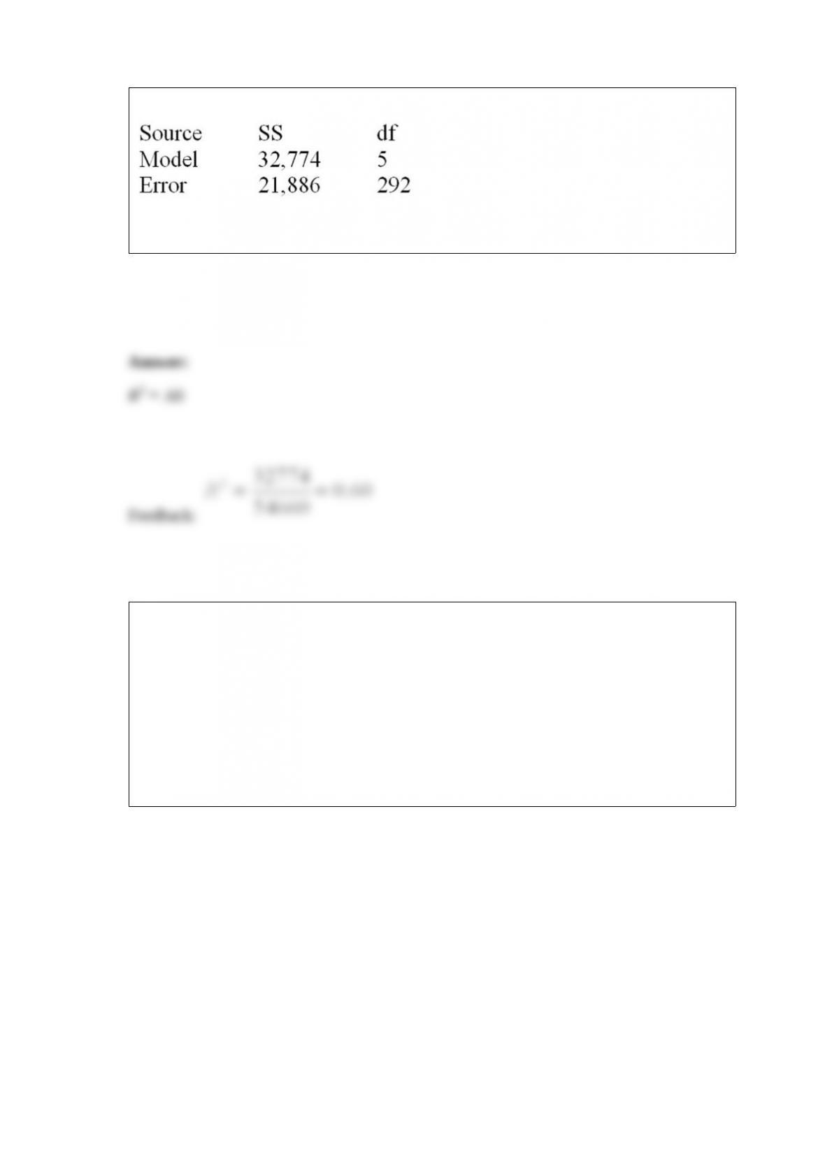
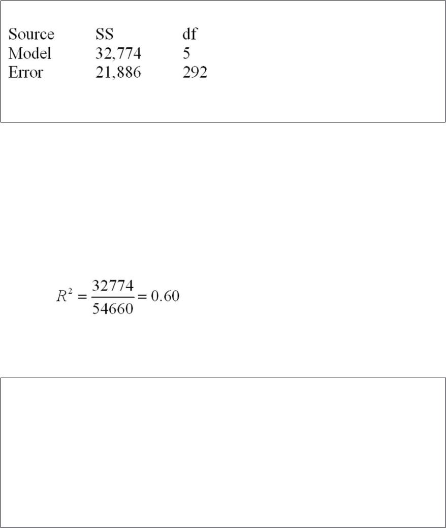
Below is a partially completed multiple regression analysis of variance (ANOVA) table.
Calculate R2.
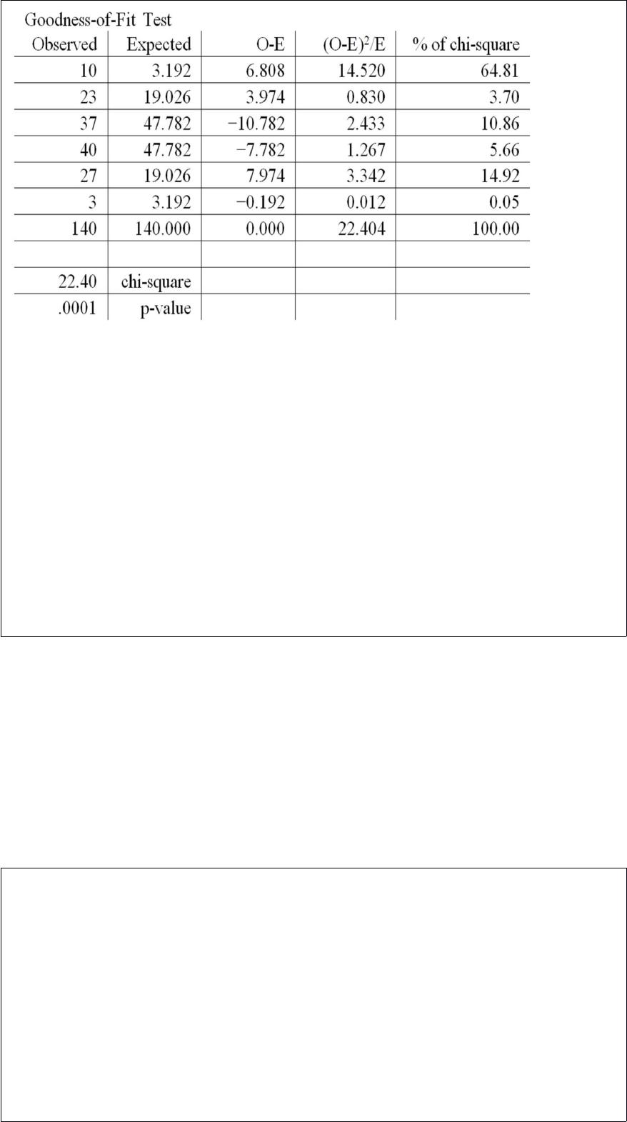
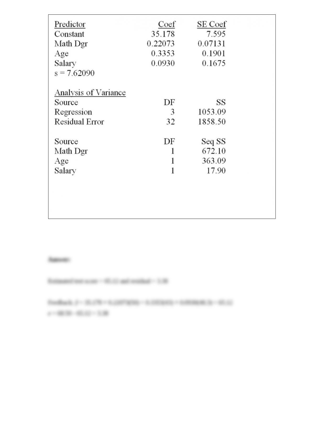
A real estate company is analyzing the selling prices of residential homes in a given
community. 140 homes that have been sold in the past month are randomly selected and
their selling prices are recorded. The statistician working on the project has stated that
in order to perform various statistical tests, the data must be distributed according to a
normal distribution. In order to determine whether the selling prices of homes included
in the random sample are normally distributed, the statistician divides the data into 6
classes of equal size and records the number of observations in each class. She then
performs a chi-square goodness-of-fit test for normal distribution. The results are
summarized in the following table.
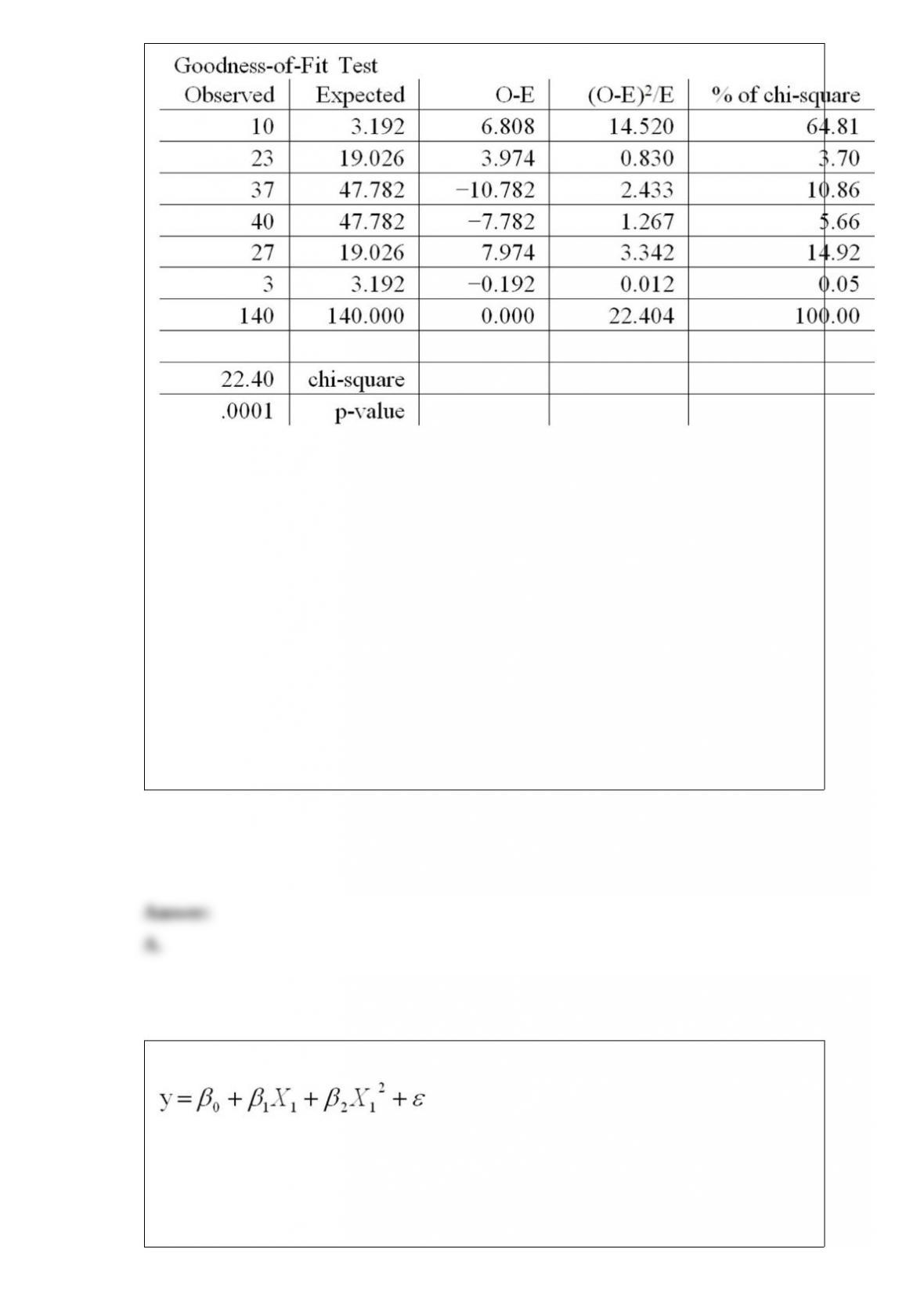
At a significance level of .05, we:
A. Reject H0; conclude the residential home selling prices are not distributed according
to a normal distribution.
B. Do not reject H0; conclude the residential home selling prices are not distributed
according to a normal distribution.
C. Reject H0; conclude the residential home selling prices are distributed according to a
normal distribution.
D. Do not reject H0; conclude the residential home selling prices are distributed
according to a normal distribution.
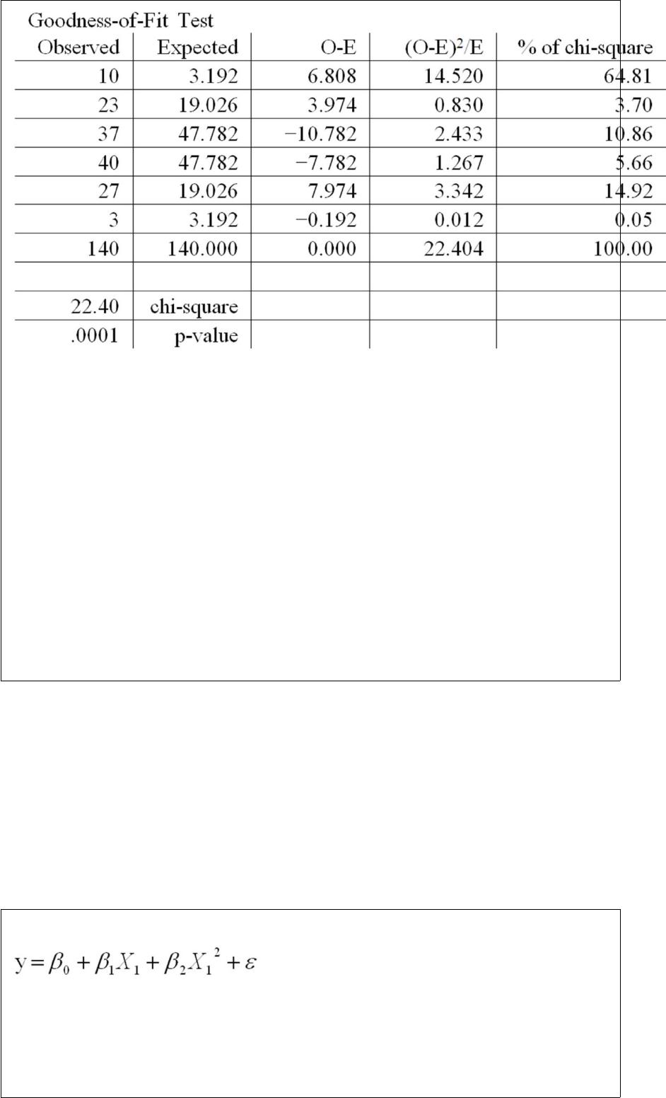
The graph of the prediction equation obtained from the model
is a(n) ____________.
A. Line
B. Plane


C. Parabola
D. Exponential curve
___________ refers to applying a treatment to more than one experimental unit.
A. Randomization
B. Balanced experiment
C. One-way ANOVA
D. Replication
In using the multiple regression method, we can model the effects of the different levels
of a qualitative independent variable by using a(n) ____________.
A. Interaction variable
B. Cross-product term
C. Quadratic term
D. Dummy (indicator) variable
E. Variance equalizing transformation
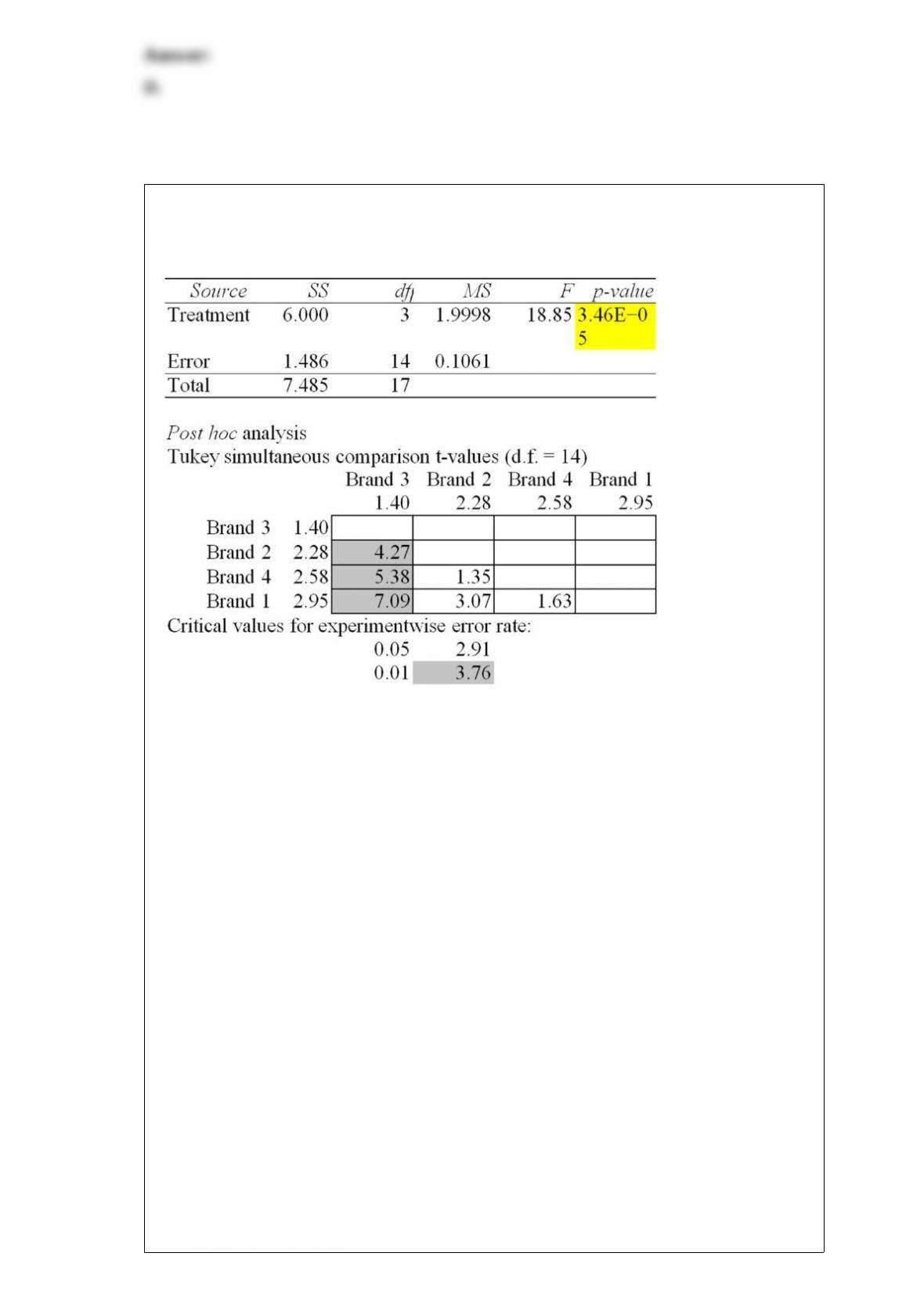
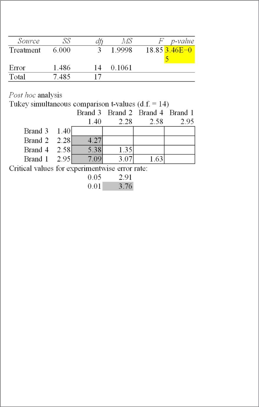
The Excel/MegaStat output given above summarizes the results of a one-way analysis
of variance in an attempt to compare the performance characteristics of four brands of
vacuum cleaners. The response variable is the amount of time it takes to clean a specific
size room with a specific amount of dirt.
At a significance level of .05, the null hypothesis for the ANOVA F test is rejected.
Analysis of the Tukey simultaneous confidence intervals shows that at the significance
level (experimentwise) of .05, we would conclude that:
A. All four brands of vacuum cleaners differ from each other in terms of their
performance.
B. Brand 1 differs from brand 2, and brand 2 differs from brand 3, while the rest of the
vacuum cleaner pairs do not differ from each other in terms of their performance.
C. Brand 1 differs from brand 2, and brand 3 differs from brands 1, 2, and 4, while the
rest of the vacuum cleaner pairs do not differ from each other in terms of their
performance.
D. Only brand 3 differs from the other three brands (brands 1, 2, and 3), while the rest
of the vacuum cleaner pairs do not differ from each other in terms of their performance.
E. None of the four brands of vacuum cleaners differ from each other in terms of their
performance.
A(n) _______ chart monitors the number of nonconforming units in a subgroup.
A.
B. R
C. C
D. p
A real estate company is analyzing the selling prices of residential homes in a given
community. 140 homes that have been sold in the past month are randomly selected and
their selling prices are recorded. The statistician working on the project has stated that
in order to perform various statistical tests, the data must be distributed according to a
normal distribution. In order to determine whether the selling prices of homes included
in the random sample are normally distributed, the statistician divides the data into 6
classes of equal size and records the number of observations in each class. She then
performs a chi-square goodness-of-fit test for normal distribution. The results are
summarized in the following table.

At a significance level of .05, what is the appropriate rejection point condition?
A. Reject H0 if χ2 > 12.5916
B. Reject H0 if χ2 > 11.0705
C. Reject H0 if χ2 > 9.3484
D. Reject H0 if χ2 > 7.81473
E. Reject H0 if χ2 > 9.48773
When the constant variance assumption holds, a plot of the residual versus x:
A. Fans out.
B. Funnels in.
C. Fans out, but then funnels in.
D. Forms a horizontal band pattern.
E. Suggests an increasing error variance.

When using simple linear regression, we would like to use confidence intervals for the
___________ and prediction intervals for the ___________ at a given value of x.
A. individual y-value, mean y-value
B. Mean y-value, individual y-value
C. Slope, mean slope
D. y-intercept, mean y-intercept
Which of the following control charts is designed to control the proportion of
nonconforming units?
A. p chart
B.
C. R chart

The number of estimated process standard deviations between and the closest
specification limit is the _____________ of the process.
A. sigma level capability
B. leeway
C. mean
D. capability
A control chart on which subgroup means are plotted versus time is a(n) _________
chart.
A.
B. R
C. p
D. C
For a given multiple regression model with three independent variables, the value of the
adjusted multiple coefficient of determination is _________ less than R2.
A. Always
B. Sometimes


C. Never
Any value of the error term in a regression model _____________ any other value of
the error term.
A. Increases with
B. Is dependent on
C. Is independent of
D. Is exactly the same as
In a multiple regression model, the residuals were plotted against the values of one of
the independent variables. The plot exhibited a funneling out pattern of residuals. This
means that as the value of the independent variable increases, the error terms tend to
___________ and the model assumption of __________ is violated.
A. increase, constant variance
B. increase, independence
C. decrease, constant variance
D. decrease, normality


In a simple linear regression analysis, the correlation coefficient (a) and the slope (b)
___________ have the same sign.
A. Always
B. Sometimes
C. Never
In performing a chi-square goodness-of-fit test for a normal distribution, if there are 7
intervals, then the degrees of freedom for the chi-square statistic is ______________.
A. 7
B. 3
C. 4
D. 6
A unit that fails to meet specifications is called a _____________ unit.


A. conforming
B. capable
C. defective
D. common cause
The chi-square goodness-of-fit test will be valid if the average of the expected cell
frequencies is ______________.
A. greater than 0
B. less than 5
C. between 0 and 5
D. at least 1
E. at least 5
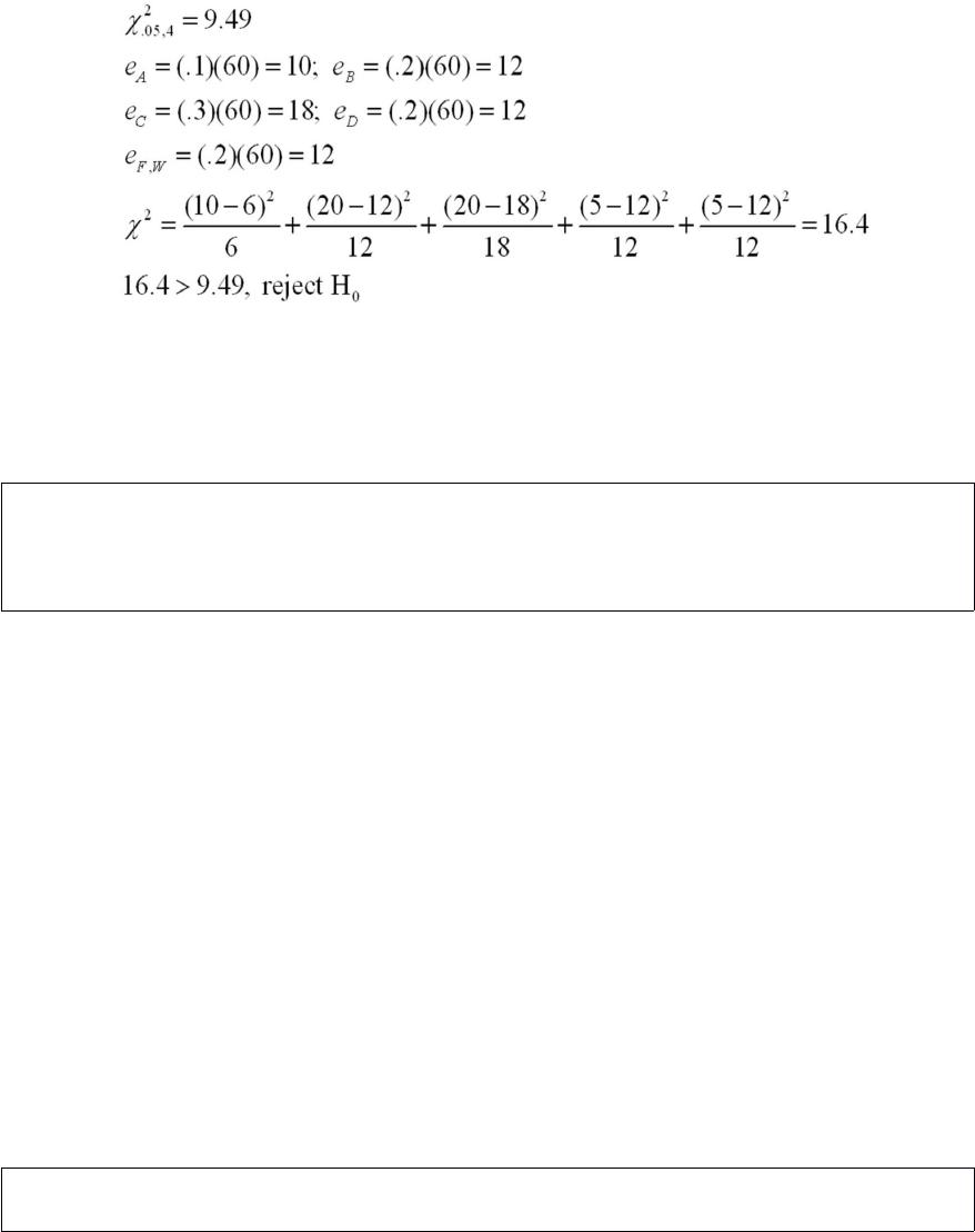
In the past, of all the students enrolled in Basic Business Statistics, 10 percent earned an
A, 20 percent earned a B, 30 percent earned a C, 20 percent earned a D, and the rest
either failed or withdrew from the course. Dr. Johnson is a new professor teaching
Basic Business Statistics for the first time this semester. At the conclusion of the
semester, of his 60 students, 10 had earned an A, 20 a B, 20 a C, 5 a D, and 5 either a W
or an F. Assume that the class constitutes a random sample. Dr. Johnson wants to know
if there is sufficient evidence to conclude that the grade distribution of his class is
different from the historical grade distribution. At α = .05, test to determine if the grade
distribution for this class is different from the historical grade distribution.
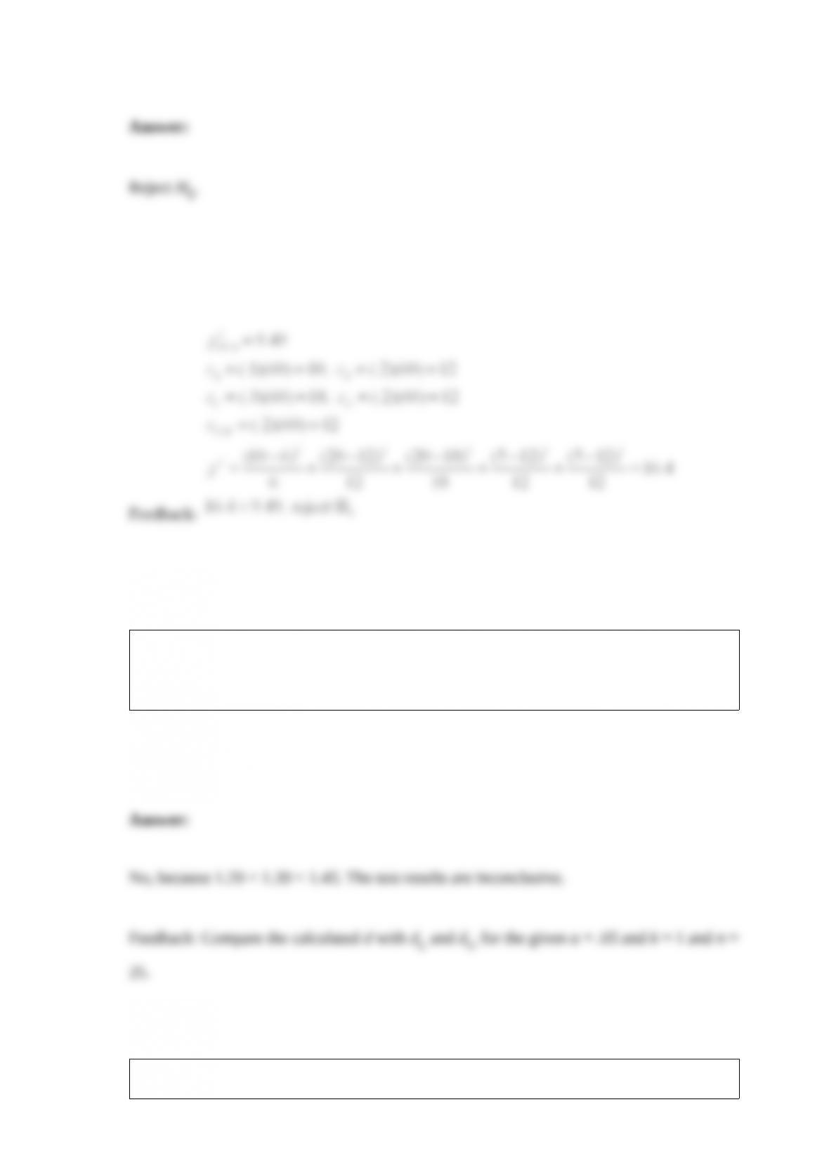
Based on 25 time-ordered observations from a simple regression model, we have
determined the Durbin-Watson statistic, d = 1.39. At α = .05, test to determine if there is
any evidence of positive autocorrelation. State your conclusions.
Below is a partial multiple regression ANOVA table.
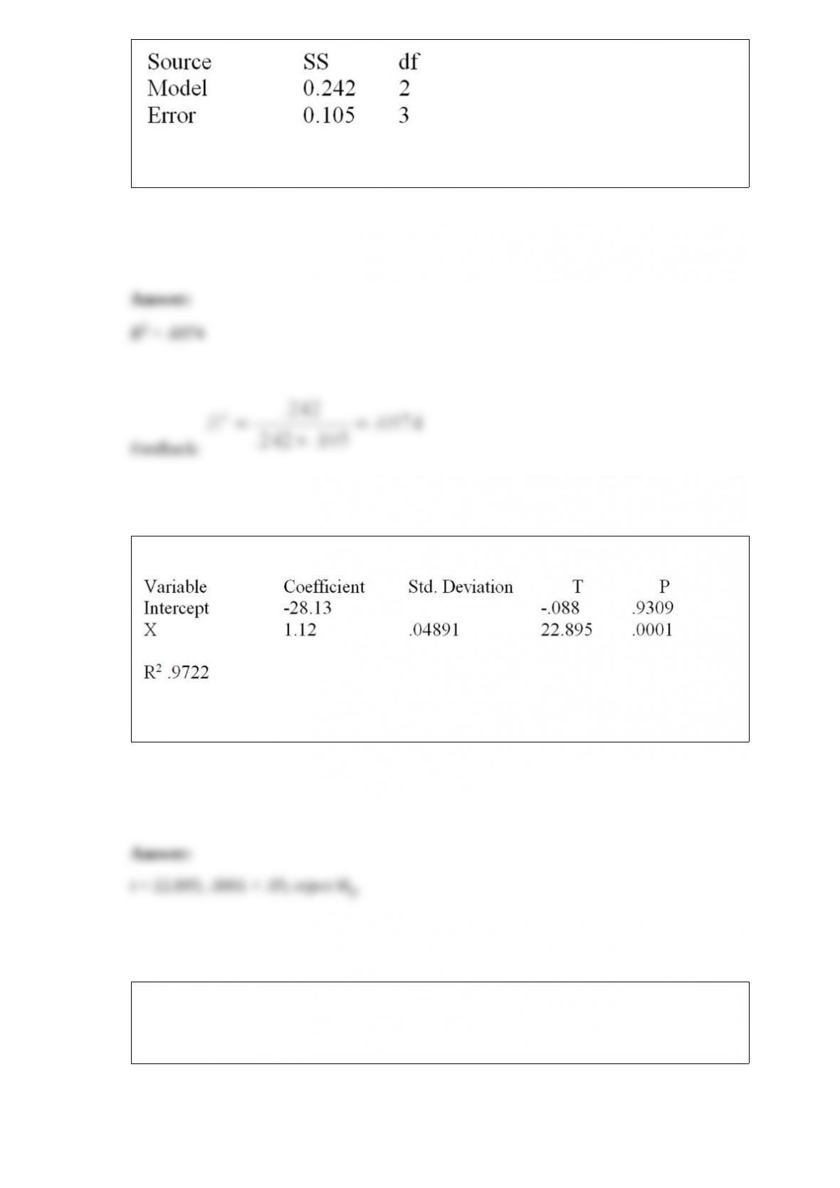
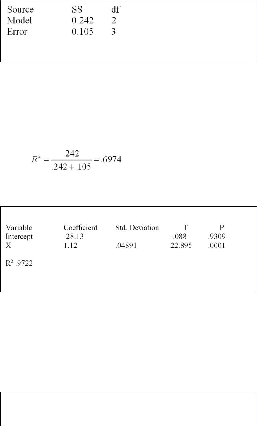
Calculate R2.
Consider the following partial computer output from a simple linear regression analysis.
Test H0: β1 ≤ 0 vs. Ha: β1 > 0.
Consider a two-way analysis of variance experiment with treatment factors A and B,
with factor A having four levels and factor B having three levels. The results are
summarized below.
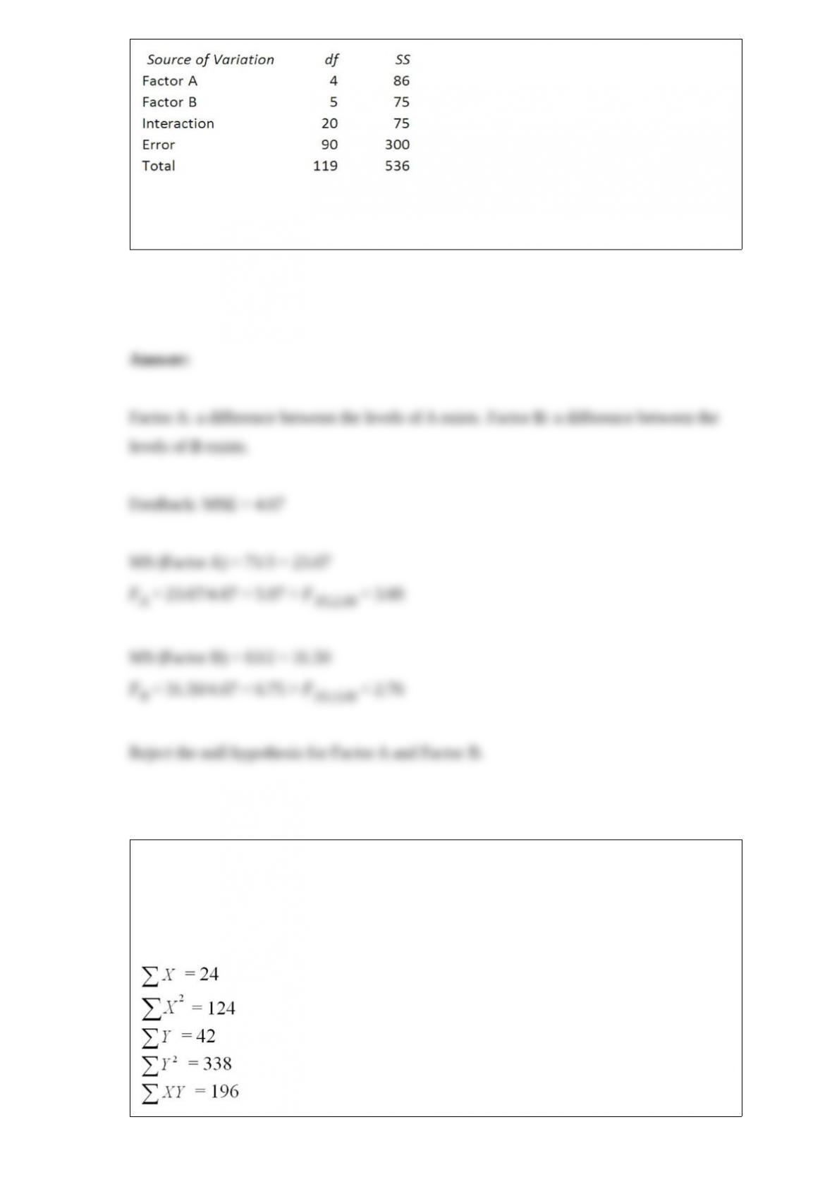
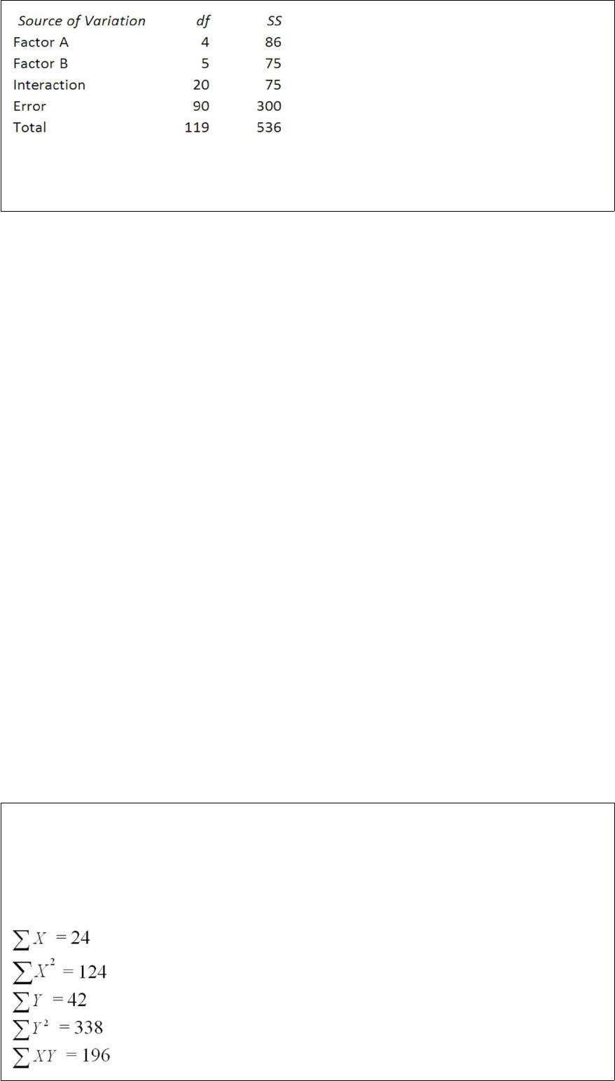
Compute the mean squares and appropriate F statistic to test the null hypotheses of no
effect from either factor at α = .05 (assumption: no interaction effect).
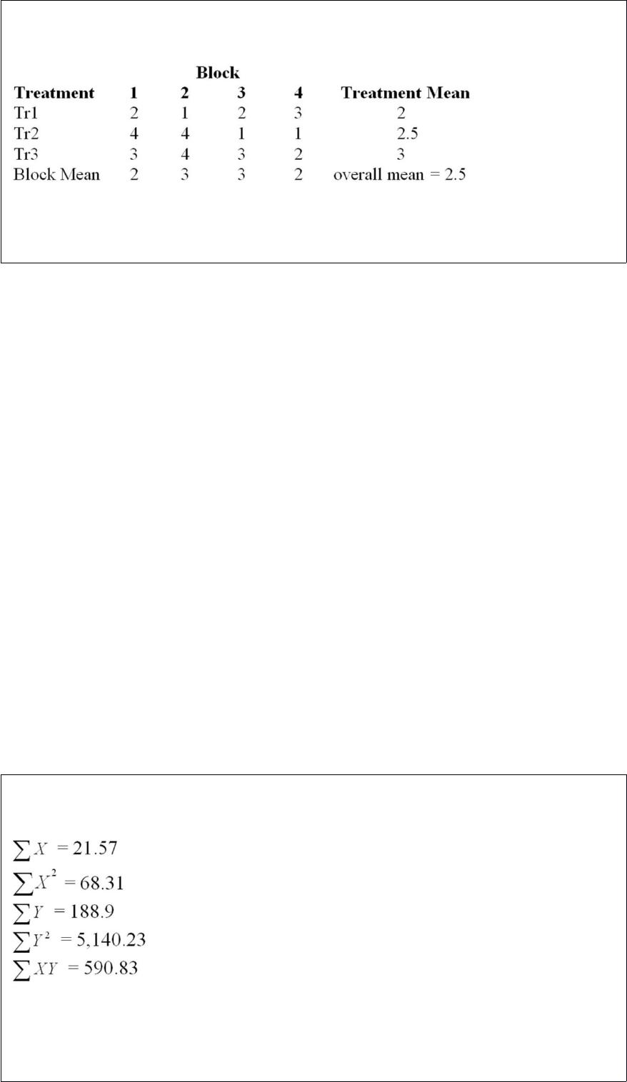
A local tire dealer wants to predict the number of tires sold each month. He believes
that the number of tires sold is a linear function of the amount of money invested in
advertising. He randomly selects 6 months of data consisting of tire sales (in thousands
of tires) and advertising expenditures (in thousands of dollars). Based on the data set
with 6 observations, the simple linear regression model yielded the following results.
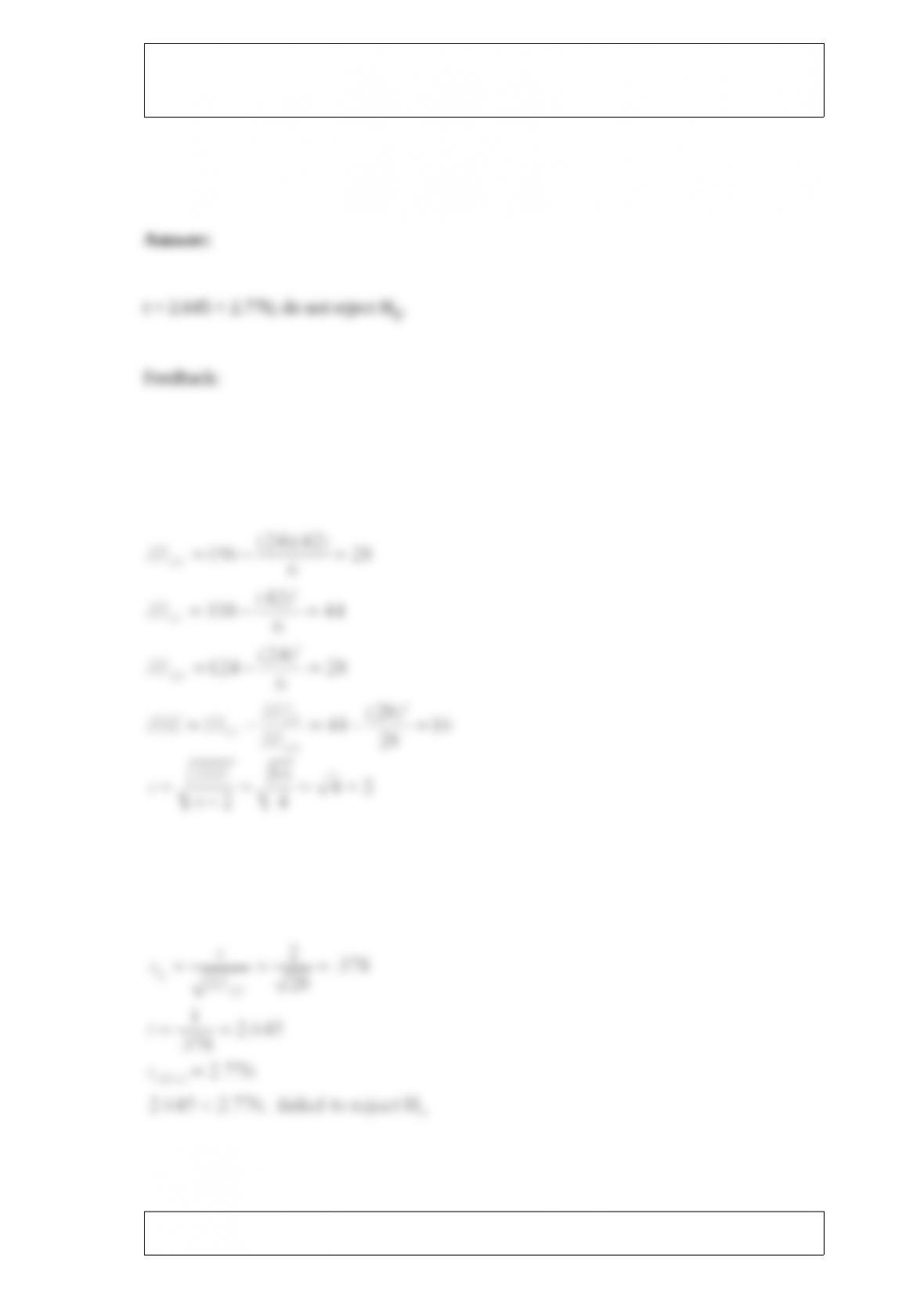
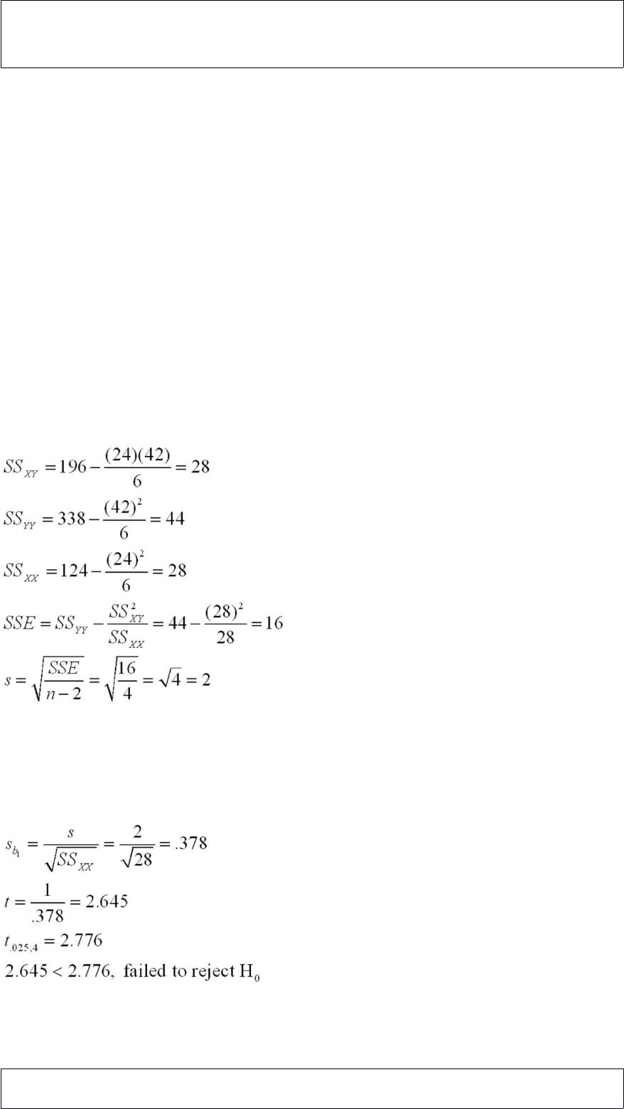
Find the rejection point for the t statistic at α = .05 and test H0: β1 = 0 vs. Ha: β1 ≠ 0.
Consider the following partial computer output from a simple linear regression analysis.
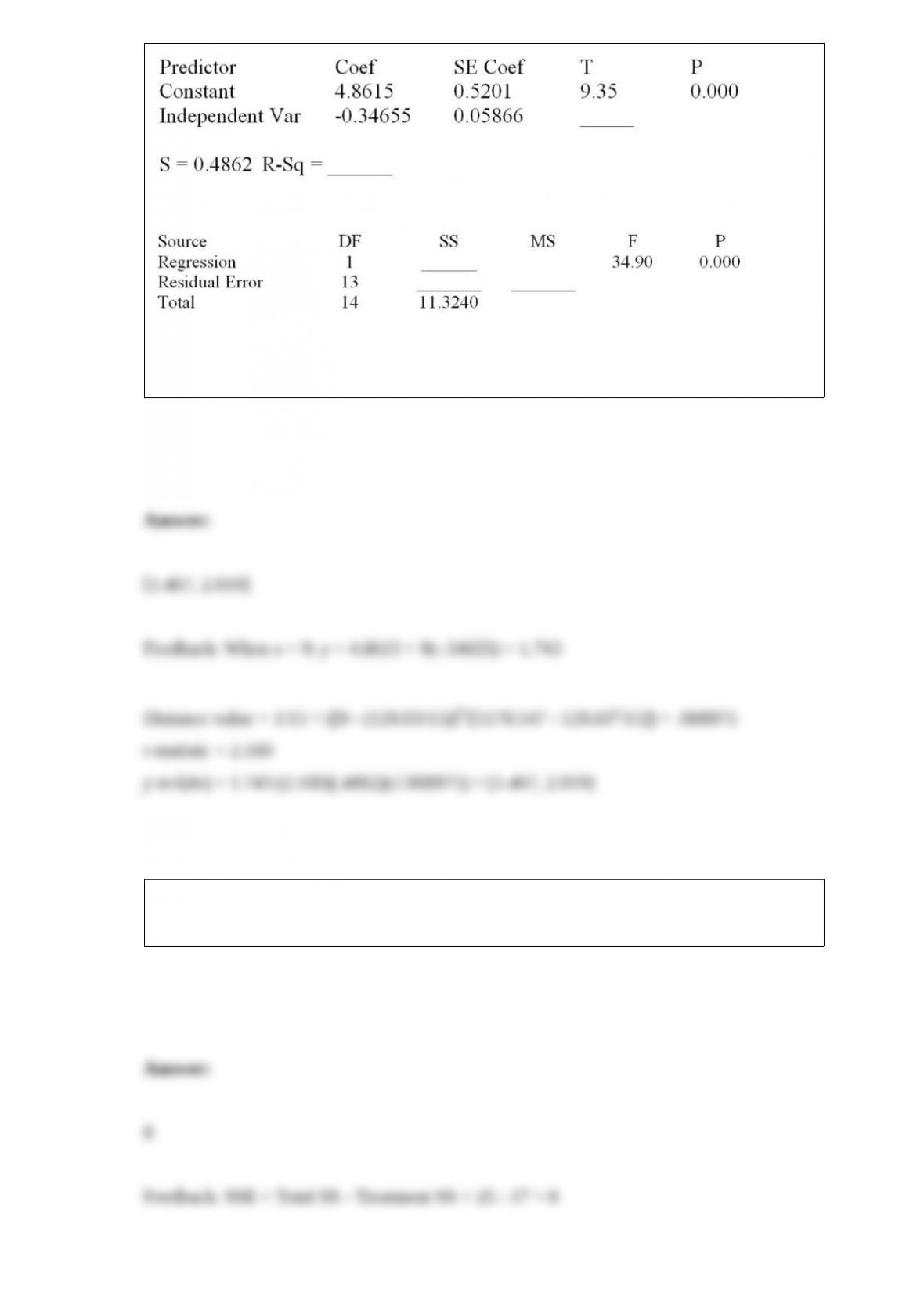
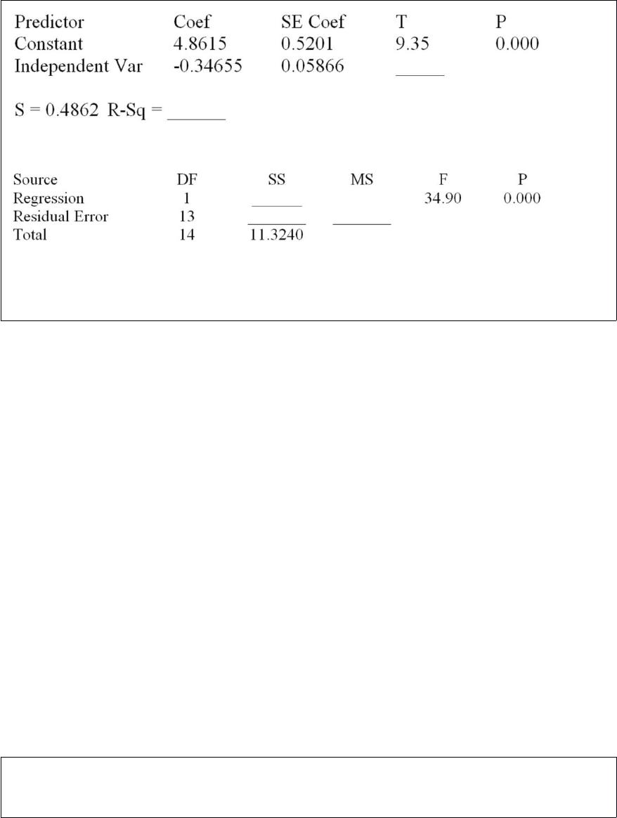
Analysis of Variance
Determine the 95 percent confidence interval for the mean value of y when x = 9.00.
Givens: ∑x = 129.03 and ∑x2 = 1178.547
If the total sum of squares in a one-way analysis of variance is 25 and the treatment sum
of squares is 17, then what is the error sum of squares?
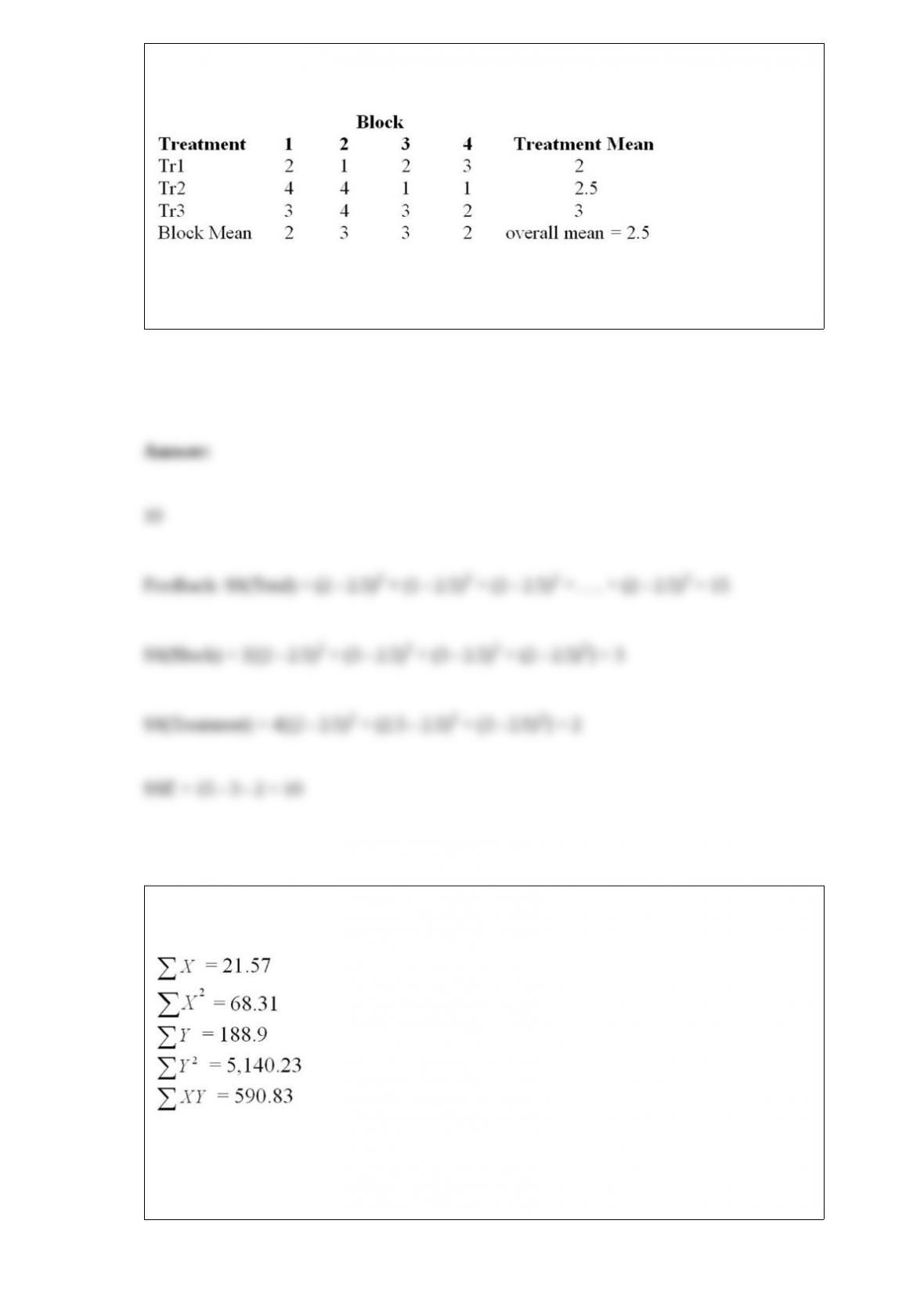
Consider the randomized block design with 4 blocks and 3 treatments given above.
What is the error sum of squares?
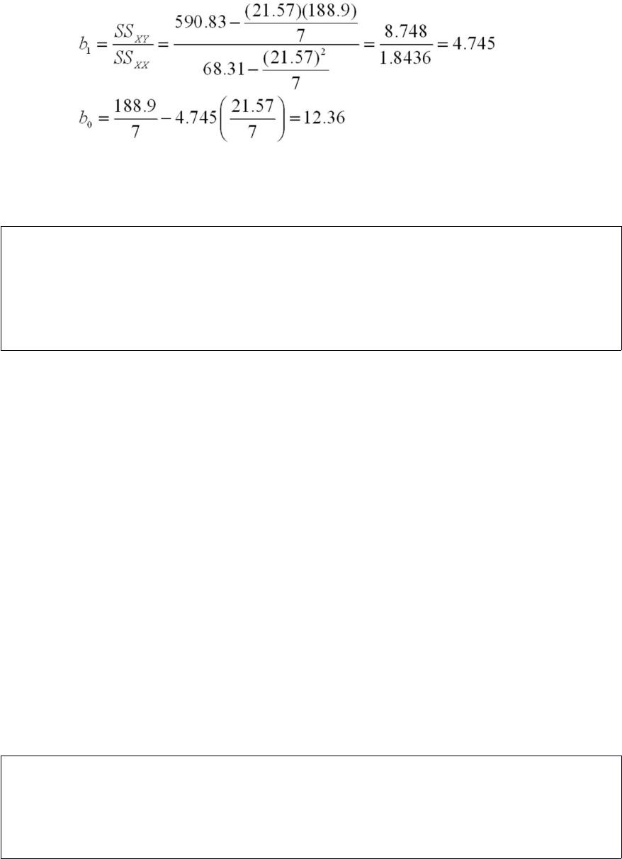
A data set with 7 observations yielded the following. Use the simple linear regression
model.
SSE = 1.117
Find the estimated y-intercept.
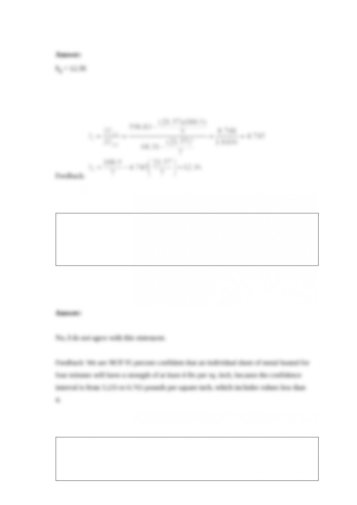
An experiment was performed on a certain metal to determine if the strength is a
function of heating time. The 95 percent prediction interval for the strength of a metal
sheet when the average heating time is 4 minutes is from 3.235 to 6.765. We are 95
percent confident that an individual sheet of metal heated for four minutes will have
strength of at least 4 pounds per square inch. Do you agree with this statement?
The manufacturer of a light fixture believes that the dollars spent on advertising, the
price of the fixture, and the number of retail stores selling the fixture in a particular
month influence the light fixture sales. The manufacturer randomly selects 10 months
and collects the following data:
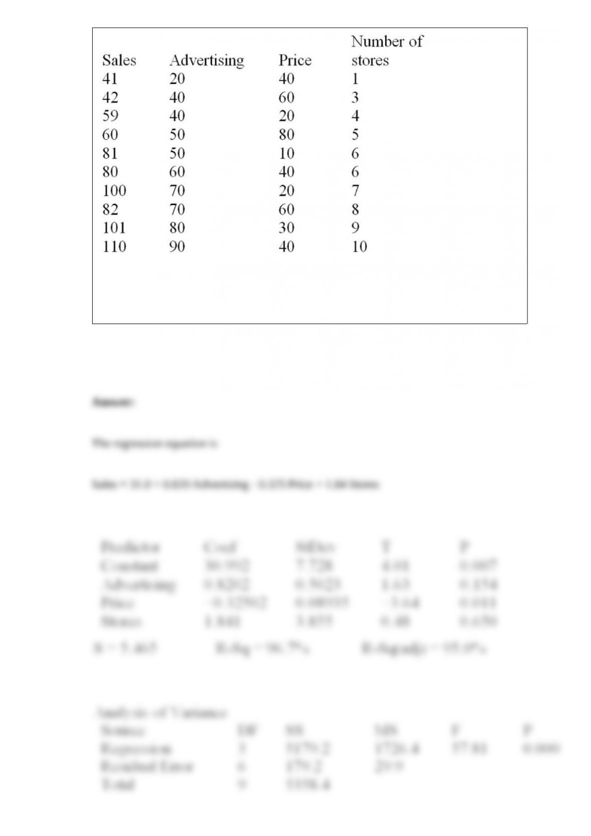
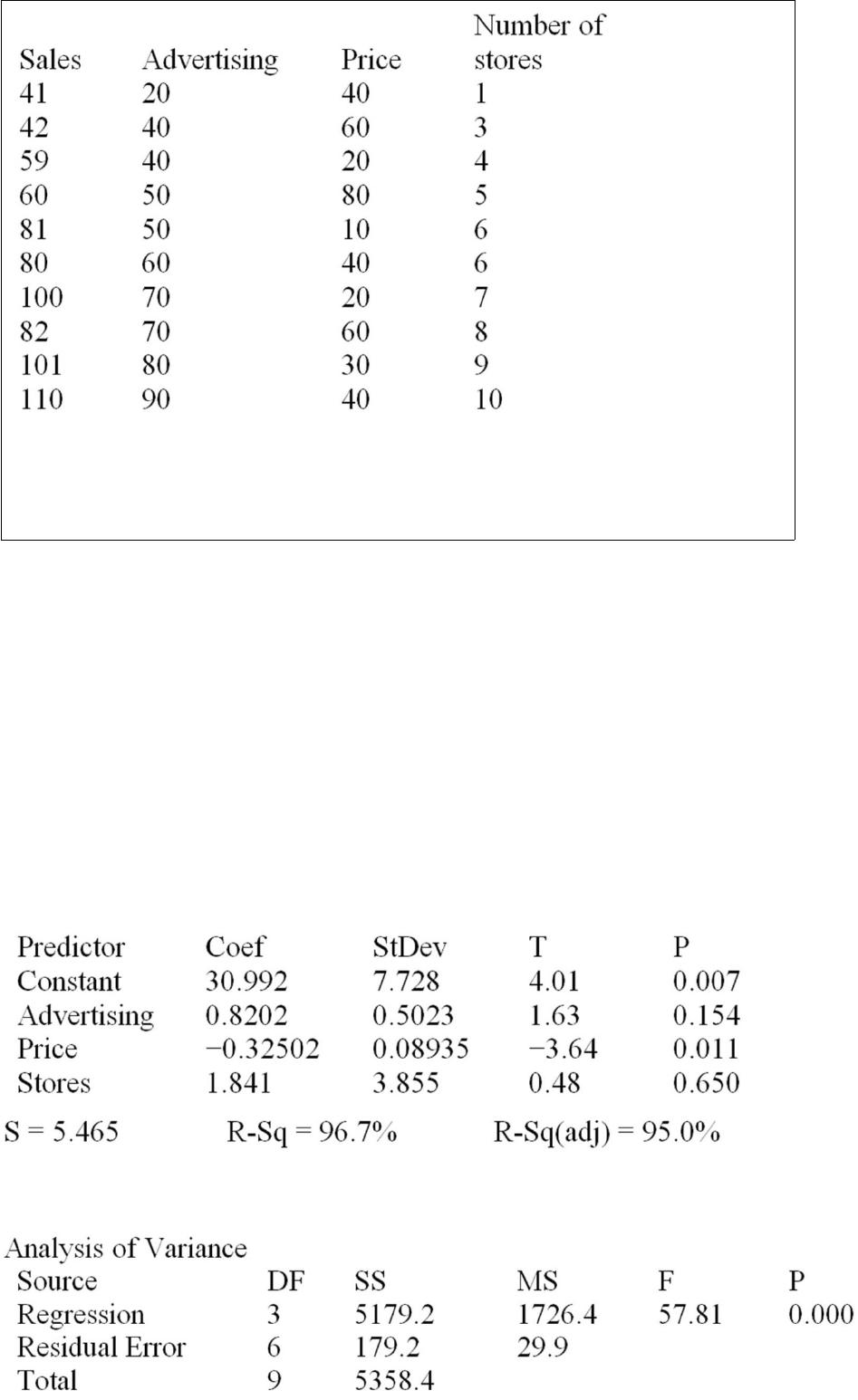
The sales are in thousands of units per month, the advertising is given in hundreds of
dollars per month, and the price is the unit retail price for the particular month. Using
MINITAB, the following computer output is obtained.
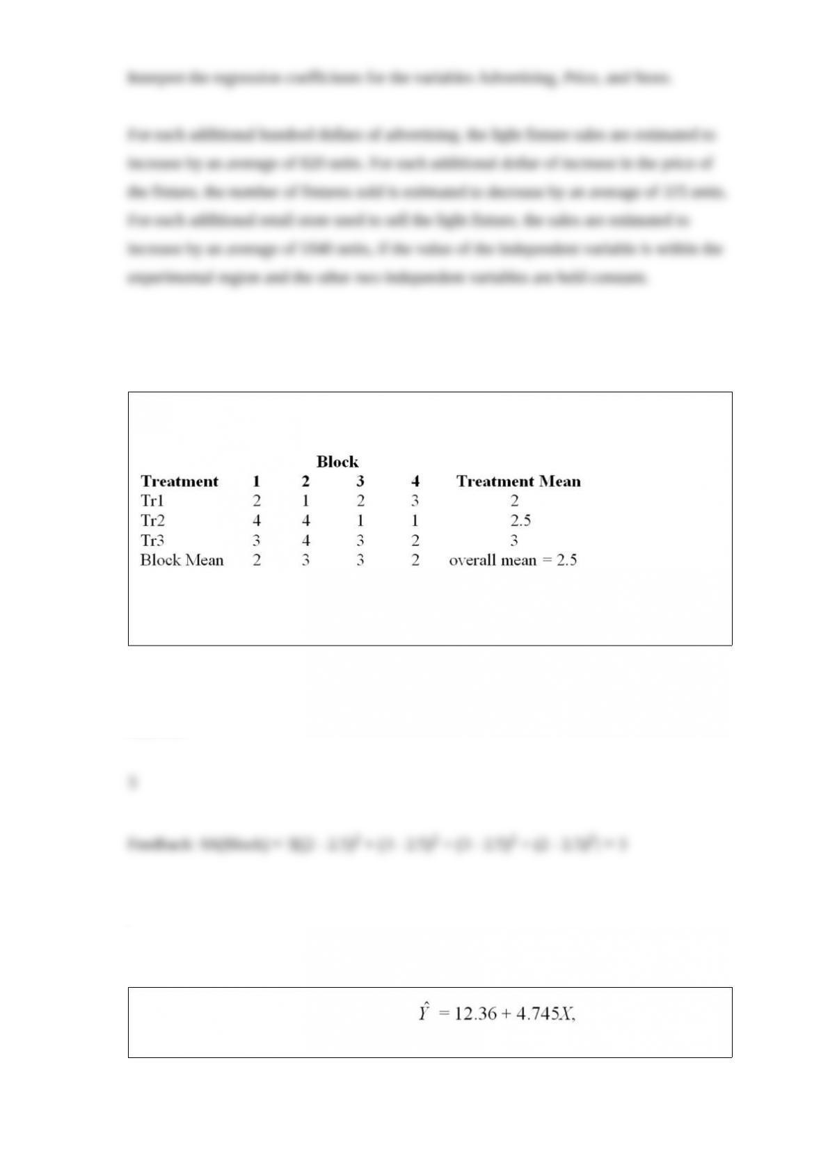
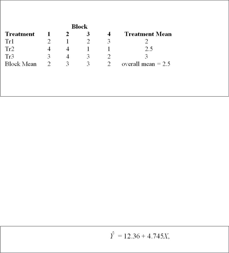
Consider the randomized block design with 4 blocks and 3 treatments given above.
What is the block sum of squares?
Use the least squares regression equation, and determine the
predicted value of y when x = 3.25.
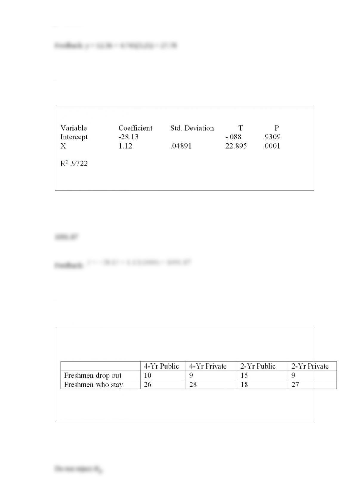
Consider the following partial computer output from a simple linear regression analysis.
What is the predicted value of y when x = 1,000?
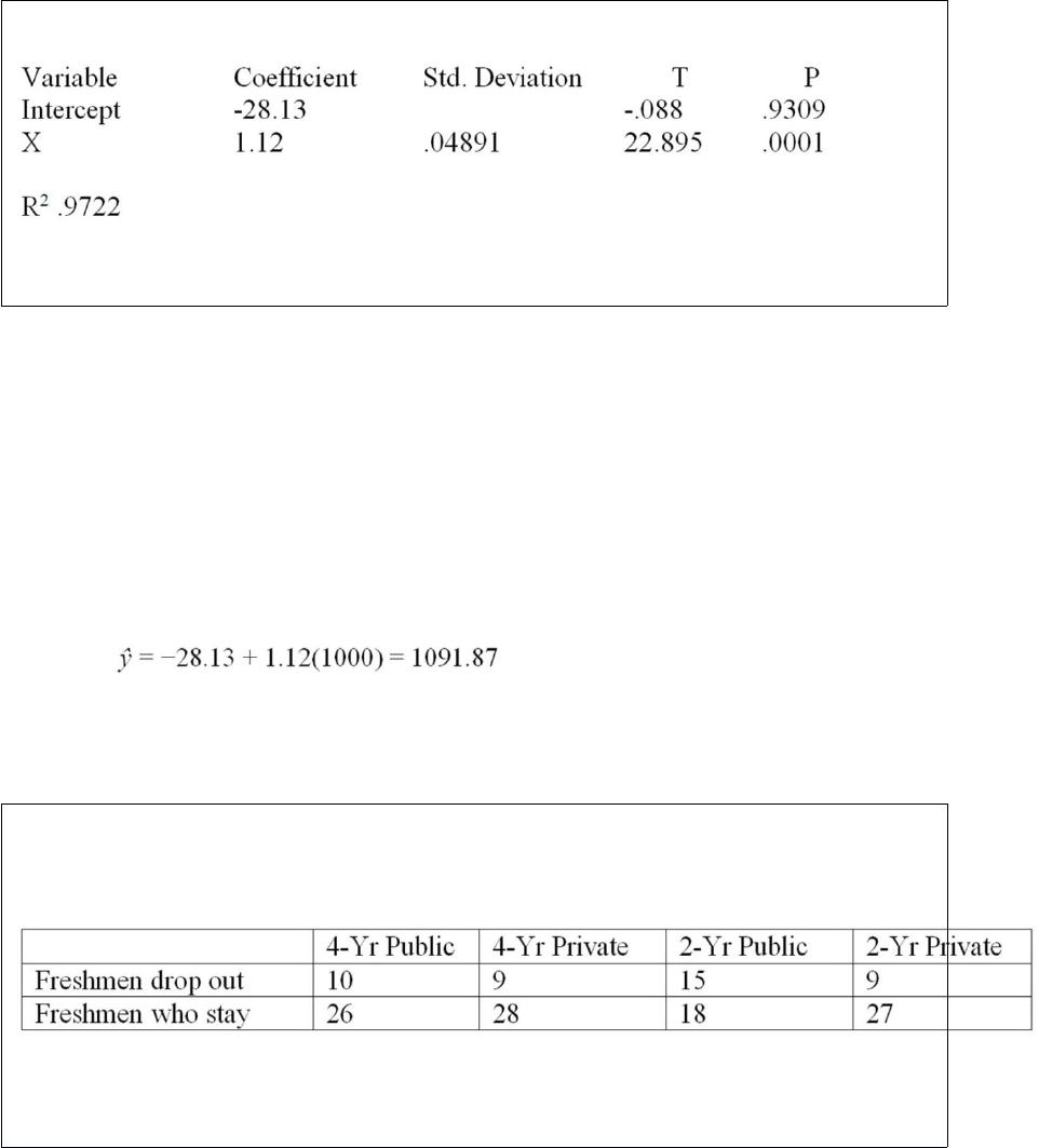
At a recent meeting of educational researchers, comparisons were made between the
type of college freshmen attend and the numbers who drop out. A random sample of
freshmen shows the following results:
Use a significance level of .05 and determine if the type of school and the drop rate are
independent. (Null hypothesis is that dropout rate is independent of type of school.)
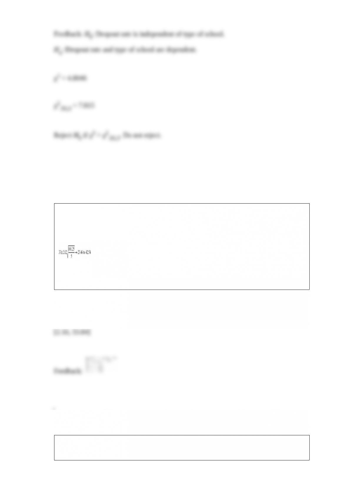
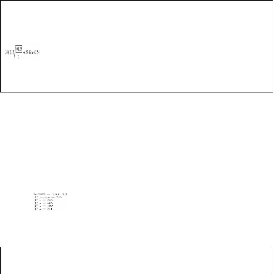
Consider the following calculations for a one-way analysis of variance from a
completely randomized design with 20 total observations. The response variable is sales
in millions of dollars, and the four treatment levels represent the four regions that the
company serves.
Perform a pairwise comparison between treatment mean 3 and treatment mean 4 by
computing a Tukey 90 percent simultaneous confidence interval.
Consider a set of 50 measurements with mean 50.2 and standard deviation 18.7 and
with the following observed frequencies.
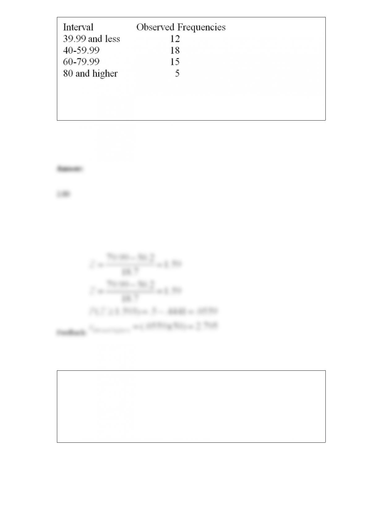
It is desired to test whether these measurements came from a normal population.
Calculate the expected frequency for the interval 80 and higher.
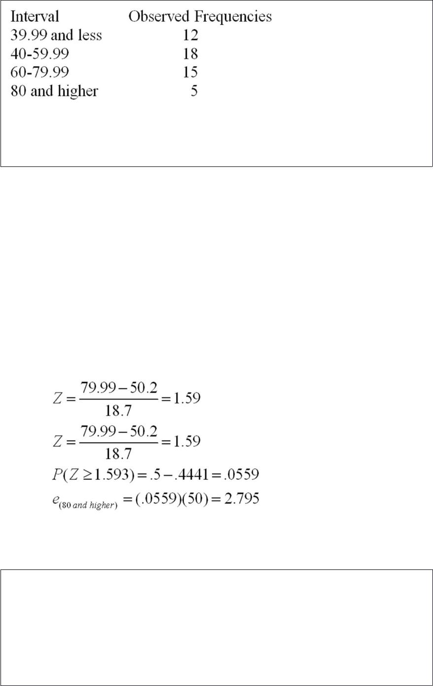
A member of the state legislature has expressed concern about the differences in the
mathematics test scores of high school freshmen across the state. She asks her research
assistant to conduct a study to investigate what factors could account for the
differences. The research assistant looks at a random sample of school districts across
the state and uses the factors of percentage of mathematics teachers in each district with
a degree in mathematics, the average age of mathematics teachers, and the average
salary of mathematics teachers.
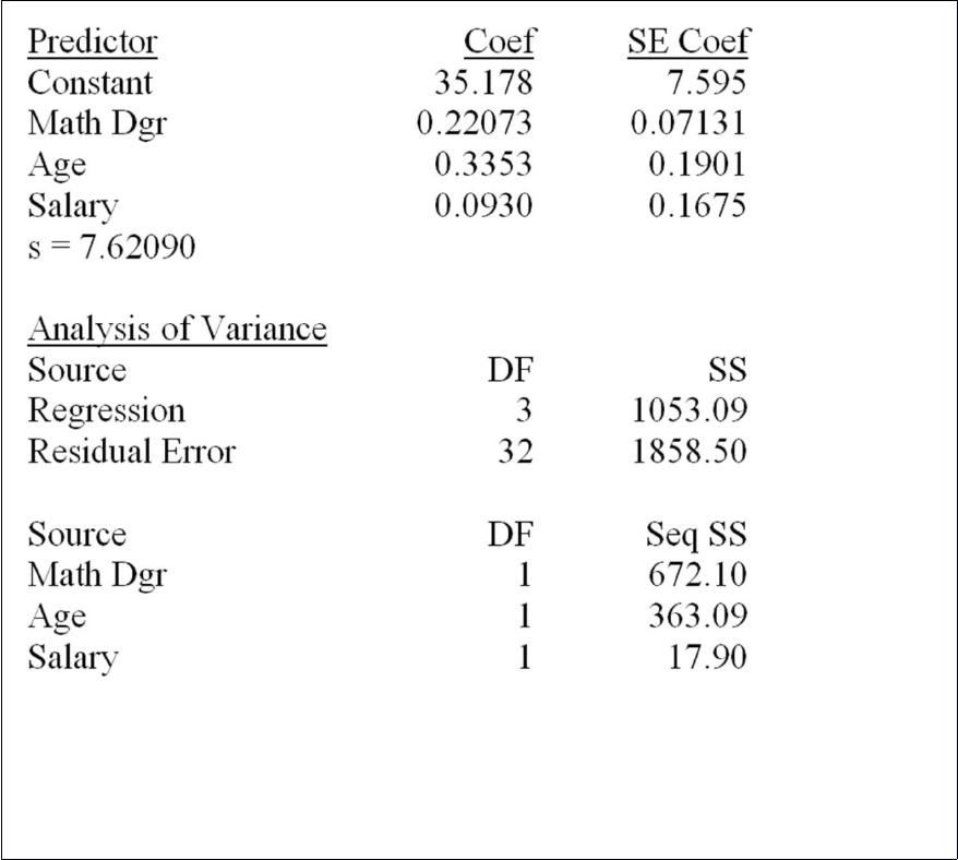
Based on the multiple regression model given above, estimate the mathematics test
score and calculate the value of the residual, if the percentage of teachers with a
mathematics degree is 50.0, the average age is 43, and the average salary is $48,300
(48.3). The actual mathematics test score for these factors is 68.50.