In a one-way analysis of variance with three treatments, each with five measurements,
in which a completely randomized design is used, what is the degrees of freedom for
error?
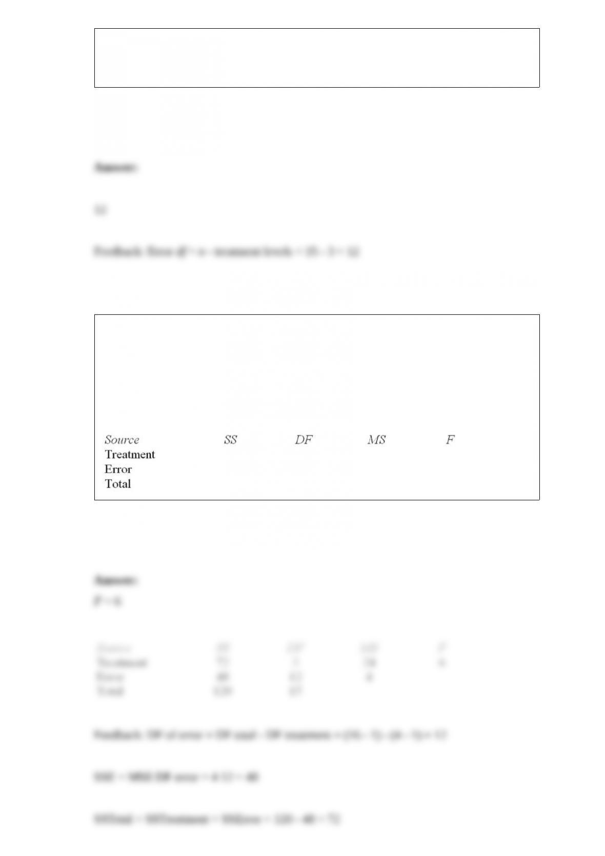
A researcher has used a one-way analysis of variance model to test whether the average
starting salaries differ among recent graduates from the nursing, engineering, business,
and education disciplines. She has randomly selected four graduates from each of the
four areas.
If MSE = 4, and SSTO = 120, complete the following ANOVA table and determine the
value of the F statistic.
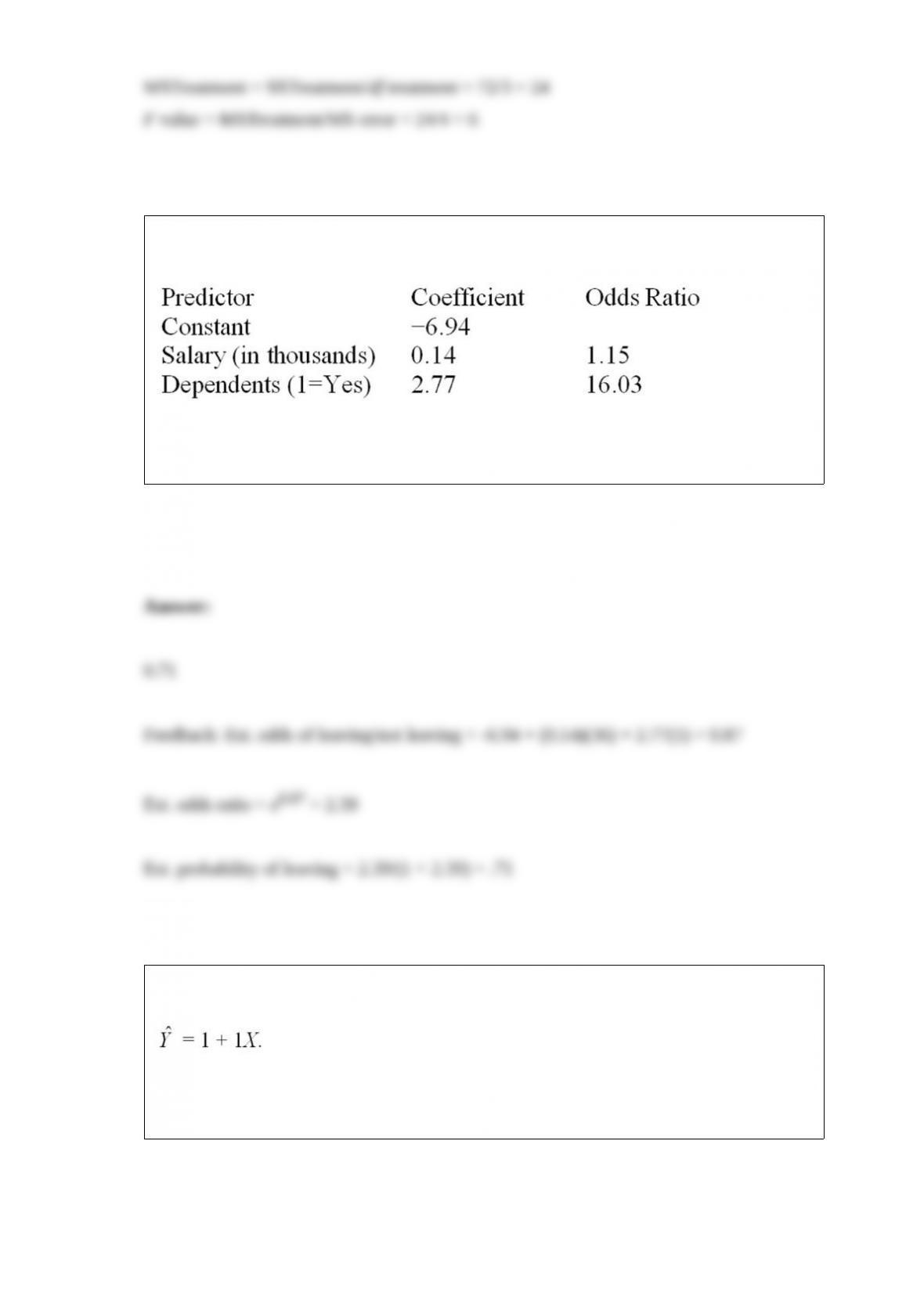
Below is a portion of a logistic regression table showing the probability of an employee
leaving his or her current position:
Estimate the probability of an employee (dependent variable) leaving his or her current
position (1 = yes) when the current salary is $36,000 and the employee has dependents.
An experiment was performed on a certain metal to determine if the strength is a
function of heating time. The simple linear regression equation is
The time is in minutes and the strength is measured in pounds per square inch. The 95
percent confidence interval for the slope is from .564 to 1.436. Can we reject β1 = 0?
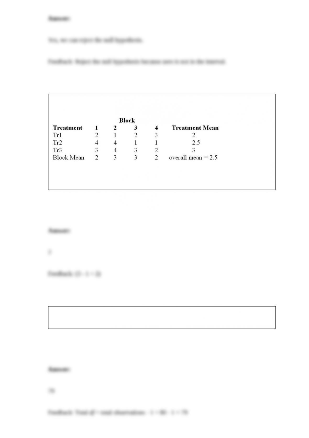
Consider the randomized block design with 4 blocks and 3 treatments given above.
What are the degrees of freedom for treatments?
Looking at four different diets, a researcher randomly assigned 20 equally overweight
women into each of the four diets. What are the degrees of freedom total?
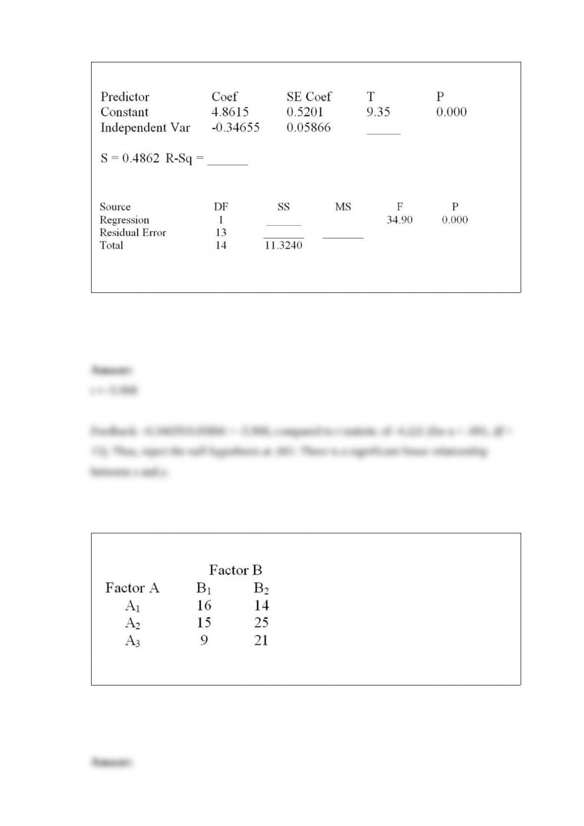
Consider the following partial computer output from a simple linear regression analysis.
Analysis of Variance
Calculate the t statistic used to test H0: β1 = 0 versus Ha: β1 ≠ 0 at α = .001.
Consider the 3 2 contingency table below.
Compute the expected frequencies in row 1.
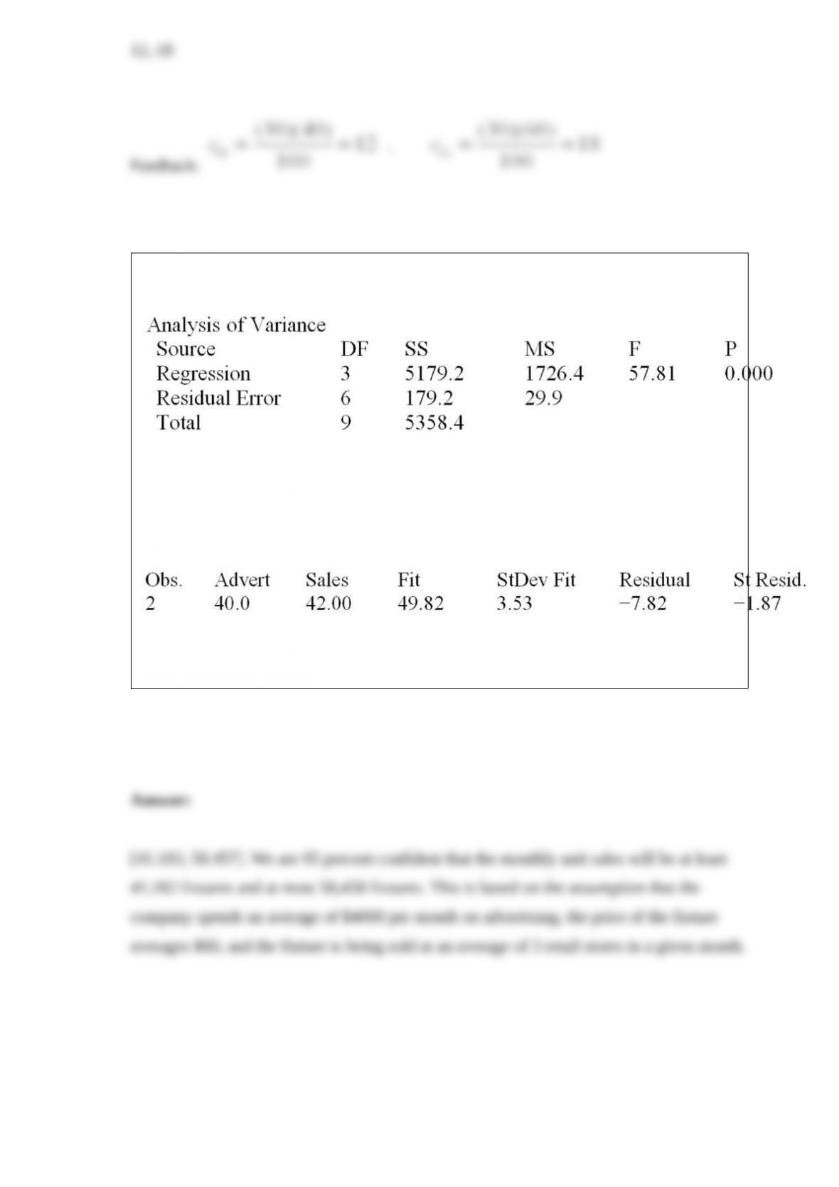
Based on the multiple regression model given above, the point estimate of the monthly
light fixture sales corresponding to second sample data is 49.82, or 49,820 units. This
point estimate is calculated based on the assumption that the company spends $4000 on
advertising, the price of the fixture is $60, and the fixture is being sold at 3 retail stores.
Additional information related to this point estimate is given below.
Determine the 95 percent confidence interval for this point estimate and interpret its
meaning.
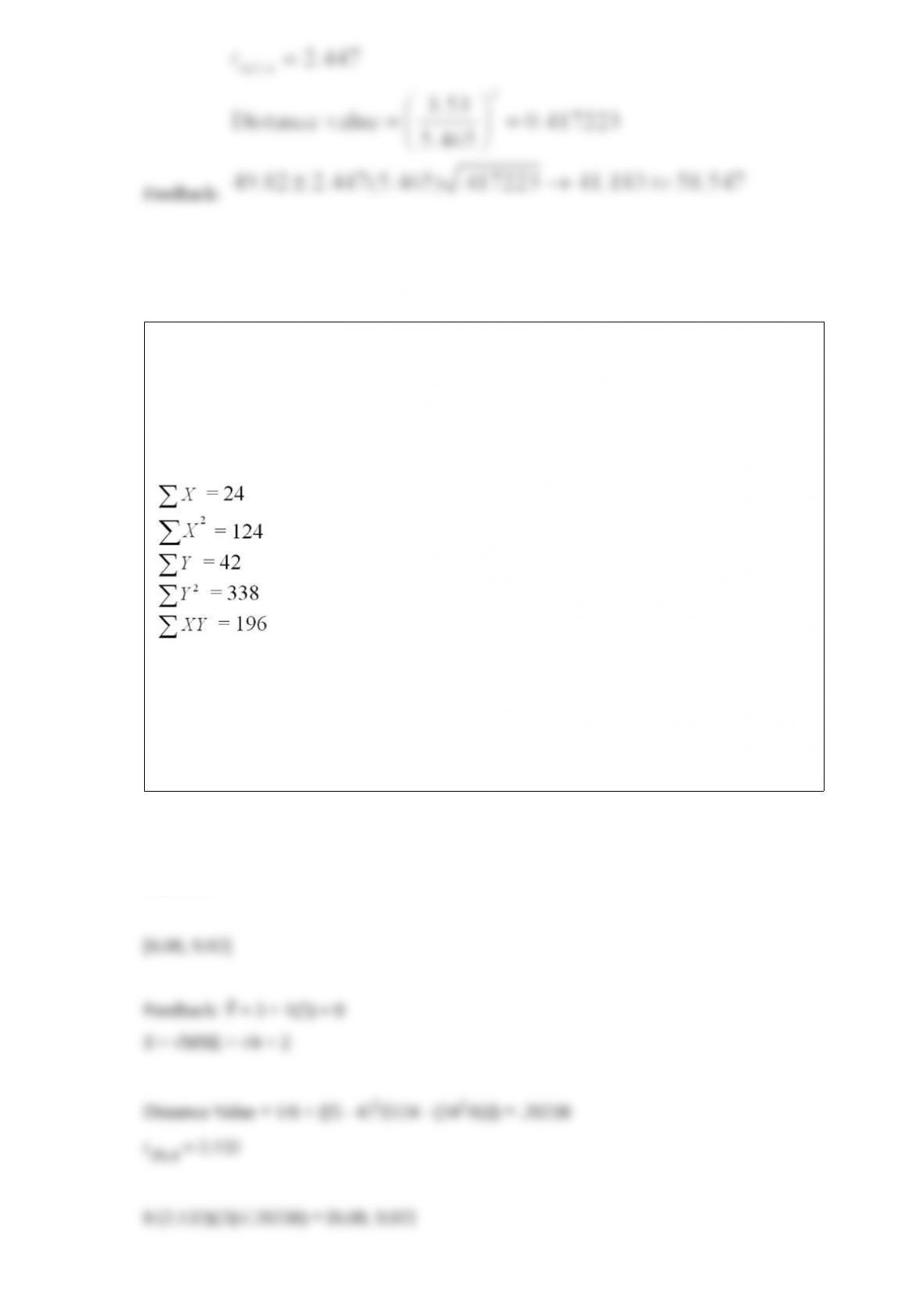
A local tire dealer wants to predict the number of tires sold each month. He believes
that the number of tires sold is a linear function of the amount of money invested in
advertising. He randomly selects 6 months of data consisting of tire sales (in thousands
of tires) and advertising expenditures (in thousands of dollars). Based on the data set
with 6 observations, the simple linear regression equation of the least squares line is ŷ =
3 + 1x.
MSE = 4
Using the sums of the squares given above, determine the 90 percent confidence
interval for the mean value of monthly tire sales when the advertising expenditure is
$5000.
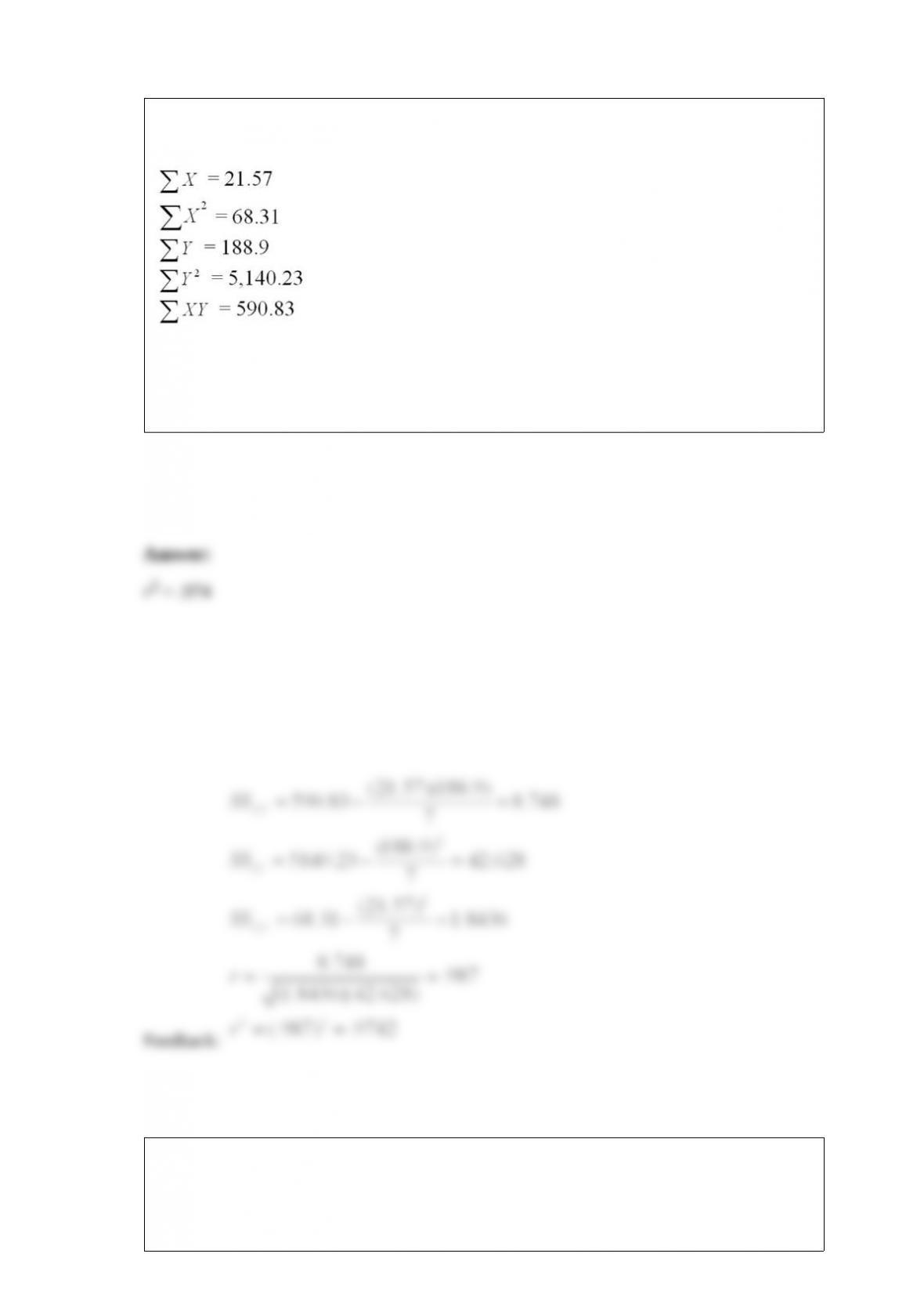
A data set with 7 observations yielded the following. Use the simple linear regression
model.
SSE = 1.117
Calculate the coefficient of determination.
A member of the state legislature has expressed concern about the differences in the
mathematics test scores of high school freshmen across the state. She asks her research
assistant to conduct a study to investigate what factors could account for the
differences. The research assistant looks at a random sample of school districts across
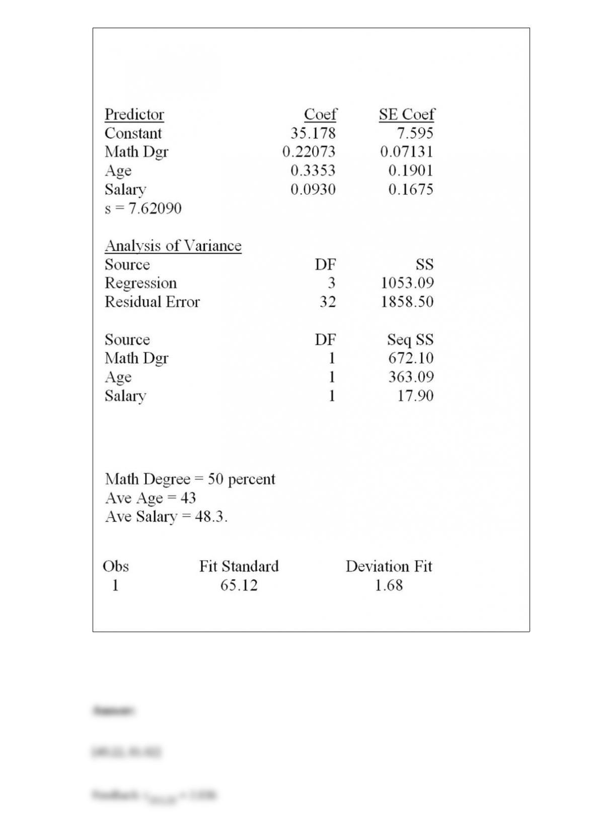
the state and uses the factors of percentage of mathematics teachers in each district with
a degree in mathematics, the average age of mathematics teachers, and the average
salary of mathematics teachers
Additional information related to this point estimate of 65.12 is given below.
Predicted Values for New Observations:
New
Calculate the 95 percent prediction interval for this point estimate.
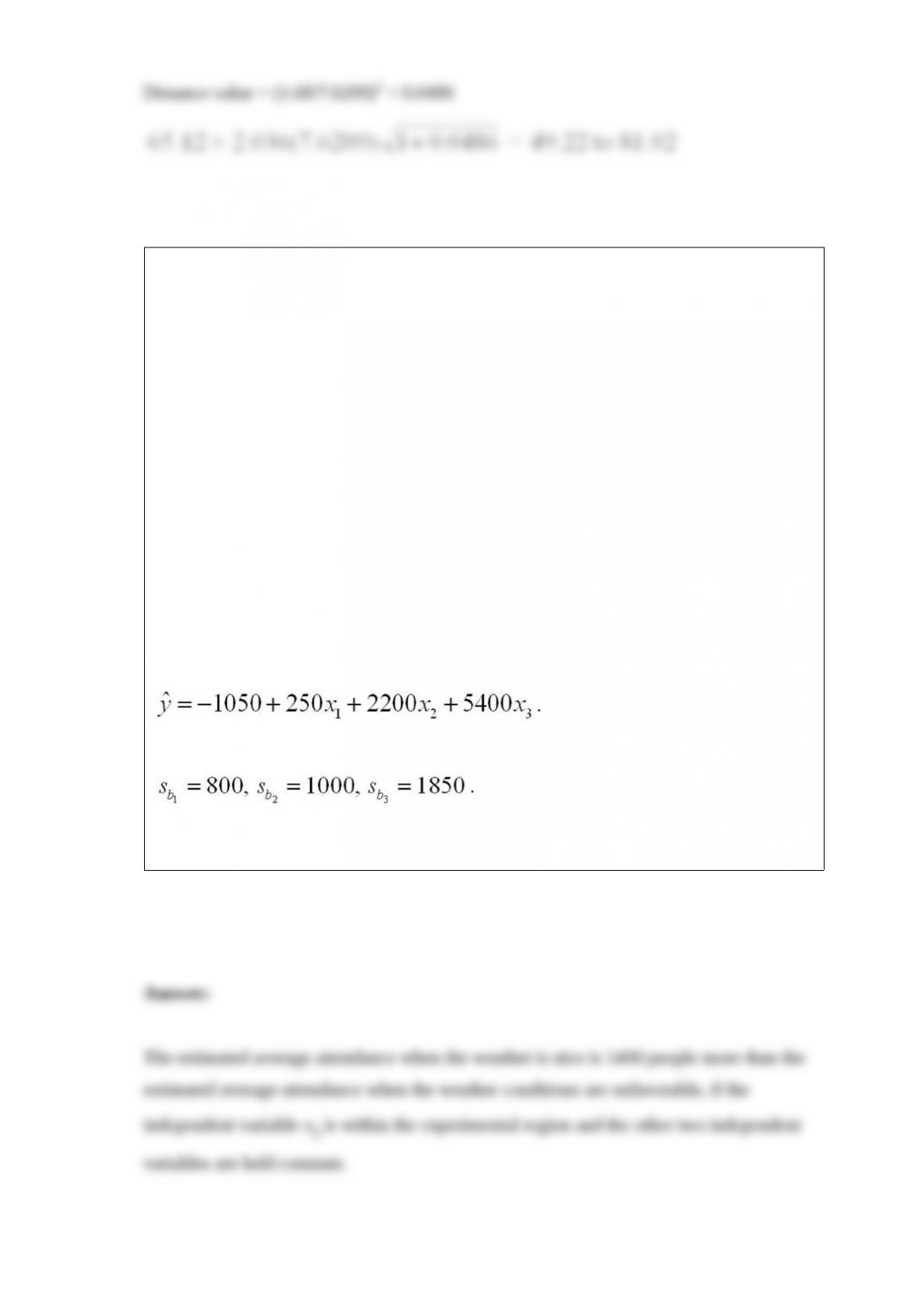
The management of a professional baseball team is in the process of determining the
budget for next year. A major component of future revenue is attendance at the home
games. In order to predict attendance at home games, the team statistician has used a
multiple regression model with dummy variables. The model is of the form y = β0 +
β1x1 + β2x2 + β3x3 + ε, where:
y = attendance at a home game.
x1 = current power rating of the team on a scale from 0 to 100 before the game.
x2 and x3 are dummy variables, and they are defined below.
x2 = 1, if weekend,
x2 = 0, otherwise.
x3 = 1, if weather is favorable,
x3 = 0, otherwise.
After collecting the data, based on 30 games from last year, and implementing the
above stated multiple regression model, the team statistician obtained the following
least squares multiple regression equation:
The multiple regression computer output also indicated the following:
Interpret the estimated model coefficient b3.
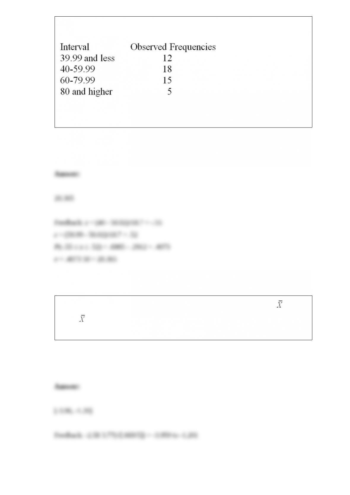
Consider a set of 50 measurements with mean 50.2 and standard deviation 18.7 and
with the following observed frequencies.
It is desired to test whether these measurements came from a normal population.
Calculate the expected frequency for the interval 40-59.99.
Find a Tukey simultaneous 95 percent confidence interval for μ1 – μ2, where 1 =
33.98, 2 = 36.56, and MSE = 0.669. There were 15 observations total and 3
treatments. Assume that the number of observations in each treatment is equal.
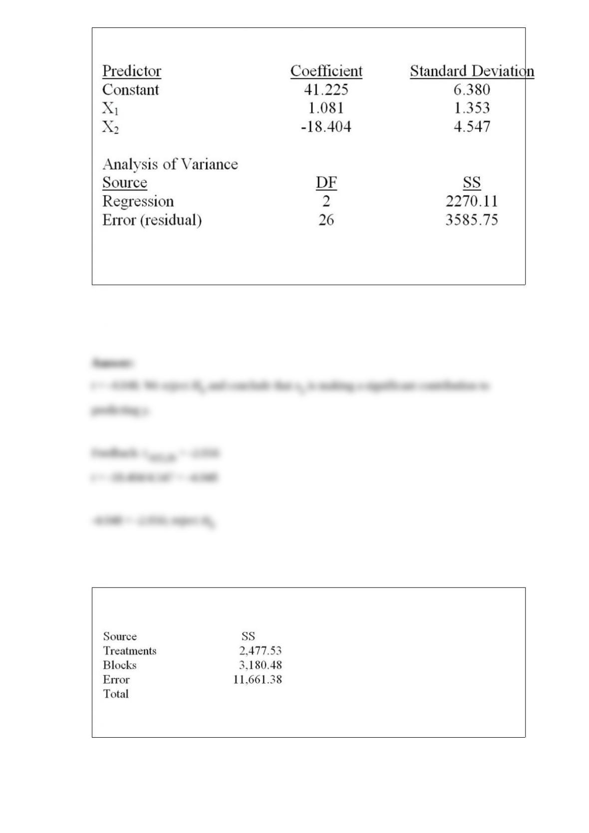
Consider the following partial computer output for a multiple regression model.
Test the usefulness of variable x2 in the model at α = .05. Calculate the t statistic and
state your conclusions.
Consider the following partial analysis of variance table from a randomized block
design with 10 blocks and 6 treatments.
What is the mean square error?