Page 61
299.
Autonomous spending occurs in the second round of spending increases caused by the
multiplier.
A)
True
B)
False
300.
Autonomous spending is an initial change in the desired level of spending by firms,
households, or government at a given level of real GDP.
A)
True
B)
False
301.
If the marginal propensity to save is 0.25 in an economy with no taxes and no imports,
the marginal propensity to consume is 1.25.
A)
True
B)
False
302.
If the marginal propensity to save is 0.25 in an economy with no taxes and no imports,
the marginal propensity to consume is 0.75.
A)
True
B)
False
303.
In an economy with no taxes or imports, if the marginal propensity to consume
increases, the marginal propensity to save will also increase.
A)
True
B)
False
304.
In an economy with no taxes or imports, if the marginal propensity to consume
increases, the marginal propensity to save will decrease.
A)
True
B)
False
305.
In an economy with no taxes or imports, if disposable income increases by $2,000 and
consumption increases by $1,400, the marginal propensity to save is 0.21.
A)
True
B)
False
Page 62
306.
In an economy with no taxes or imports, if disposable income decreases by $2,000 and
consumption decreases by $1,400, the marginal propensity to save is 0.3.
A)
True
B)
False
307.
In an economy with no taxes or imports, if disposable income decreases by $2,000 and
consumption decreases by $1,400, the multiplier is 7.
A)
True
B)
False
308.
In an economy with no taxes or imports, if disposable income decreases by $2,000 and
consumption decreases by $1,500, the marginal propensity to consume is –0.25.
A)
True
B)
False
309.
In an economy with no taxes or imports, if disposable income decreases by $2,000 and
consumption decreases by $1,500, the multiplier is –4.
A)
True
B)
False
310.
In an economy with no taxes and no imports, disposable income increases from $1,000
to $2,000. If consumption increases from $800 to $1500, the marginal propensity to
consume is 0.7.
A)
True
B)
False
311.
In an economy with no taxes and no imports, disposable income increases from $1,000
to $2,000. If consumption increases from $800 to $1,500, the marginal propensity to
save is 0.25.
A)
True
B)
False
312.
In an economy with no taxes and no imports, disposable income increases from $1,000
to $2,000. If consumption increases from $800 to $1,500, the marginal propensity to
save is 0.3.
A)
True
B)
False
Page 63
313.
In an economy with no taxes and no imports, disposable income increases from $1,000
to $2,000. If consumption increases from $800 to $1,500, the multiplier is 3.33.
A)
True
B)
False
314.
If the marginal propensity to consume decreases, the multiplier will increase.
A)
True
B)
False
315.
If the marginal propensity to save decreases, the multiplier will increase.
A)
True
B)
False
316.
If the marginal propensity to consume is 0.9, the multiplier will be 0.1.
A)
True
B)
False
317.
If the marginal propensity to save is 0.2, the multiplier will be 5.
A)
True
B)
False
318.
If the marginal propensity to consume is 0.9 and investment spending increases by $50
billion, the change in real GDP will be $5 billion.
A)
True
B)
False
319.
If the marginal propensity to save is 0.25 and investment spending increases by $50
billion, the change in real GDP will be $200 billion.
A)
True
B)
False
320.
If the consumption function is C = $100 million + 0.8* YD, then the marginal propensity
to consume is $100 million.
A)
True
B)
False
Page 64
321.
The marginal propensity to consume is consumption divided by disposable income.
A)
True
B)
False
322.
If you expect to get a substantial raise six months from now and if you are like most
people, it will not affect your current consumption because you haven’t received the
money yet.
A)
True
B)
False
323.
The aggregate consumption function can shift because of changes in expected
disposable income and in aggregate wealth.
A)
True
B)
False
324.
According to the life-cycle hypothesis, consumers plan their spending based on their
current disposable income when they are very young.
A)
True
B)
False
325.
People use wealth to smooth consumption over their life cycle.
A)
True
B)
False
326.
Planned investment spending is inversely related to the interest rate, because fewer
projects are profitable at higher interest rates.
A)
True
B)
False
327.
If expected GDP increases, then current planned investment will increase.
A)
True
B)
False
328.
The higher current production capacity is, the higher current planned investment will be.
A)
True
B)
False
Page 65
329.
Planned investment spending and actual investment spending are NOT always equal.
A)
True
B)
False
330.
If planned investment is $50 billion and unplanned inventory investment is $10 billion,
then actual investment is $40 billion.
A)
True
B)
False
331.
Inventories are counted as investment because inventories are a source of future sales.
A)
True
B)
False
332.
If real GDP is greater than planned expenditure, unplanned inventory investment is
negative.
A)
True
B)
False
333.
Changes in unplanned inventory investment move the economy toward the
Income–Expenditure equilibrium.
A)
True
B)
False
334.
Decreases in investment spending are usually offset by increases in consumption
through the multiplier process.
A)
True
B)
False
335.
If planned aggregate spending rises by $10 billion and the marginal propensity to
consume is 0.8, then the income–expenditure equilibrium increases by 50 billion.
A)
True
B)
False
336.
If planned aggregate spending rises by $20 billion and the marginal propensity to
consume is 0.9, then the income–expenditure equilibrium increases by $18 billion.
A)
True
B)
False

Page 66
337.
The main cause of the recession that ended in late 2001 was a decrease in consumer
savings.
A)
True
B)
False
338.
An increase in consumer spending on durable goods was the main factor that ended the
recession in 2001.
A)
True
B)
False
339.
Negative inventory investment caused the growth of GDP to be fairly low when the
recovery from the recession began in the fourth quarter of 2001.
A)
True
B)
False
340.
Explain how Finland’s real GDP per capita in 2016 falling by almost 10% from its peak
in 2008 illustrates the positive and negative effects of the multiplier.
341.
Suppose that the marginal propensity to consume is 0.80 and the government spends
$10 million to repair a bridge. Assuming no taxes and no international trade, explain
how the $10 million of government spending will increase GDP by $50 million.
342.
How does a nation’s savings rate, as measured by the marginal propensity to save, affect
the size of the spending multiplier?
343.
How can autonomous consumption be greater than zero when disposable income equals
zero?
344.
Suppose you have estimated the consumption function as C = 250 + 0.90* YD. What is
the equation for the corresponding savings function?
Page 67
Use the following to answer question 345:
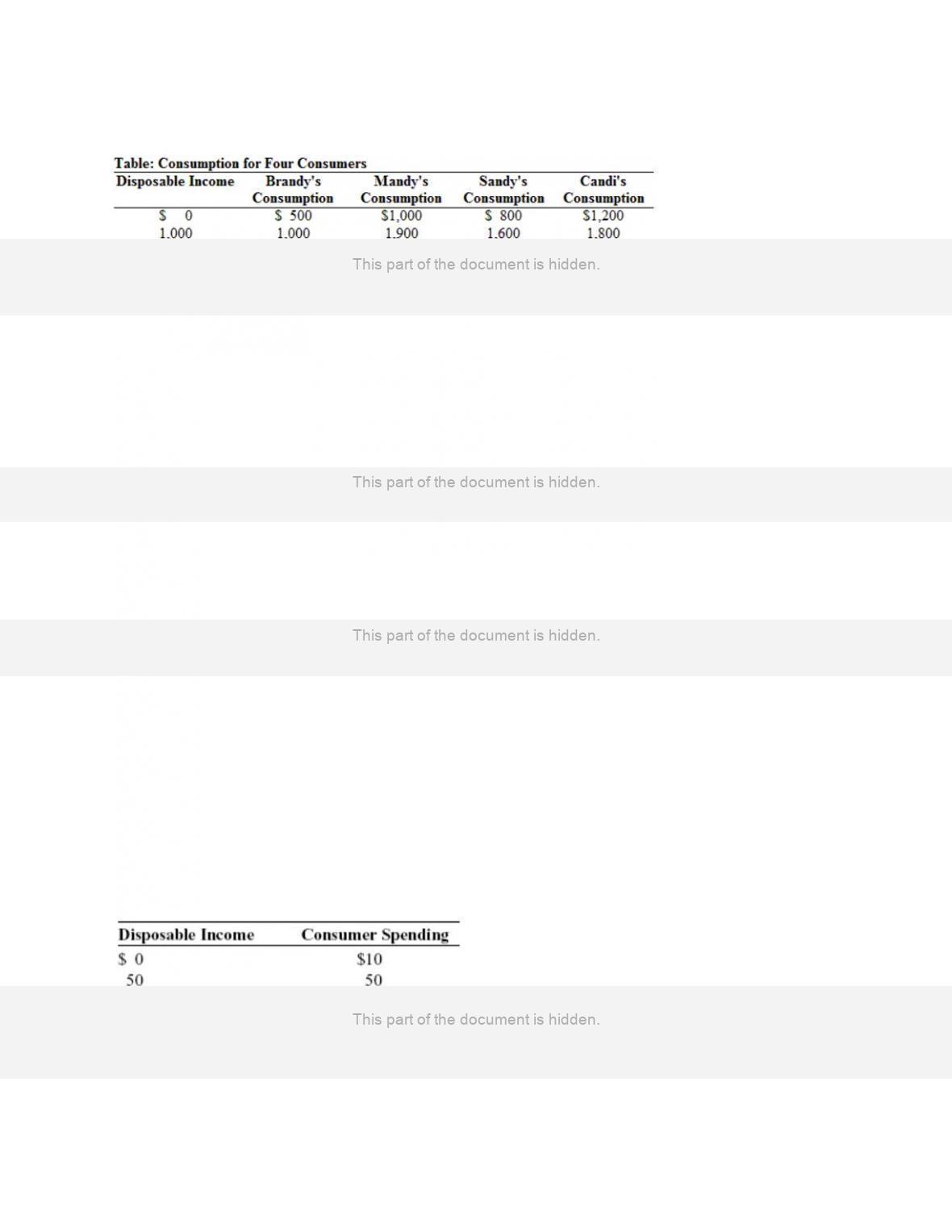
345.
(Table: Consumption for Four Consumers) Use Table: Consumption for Four
Consumers. Construct the aggregate consumption function.
346.
Suppose the economy is in income–expenditure equilibrium. How will each of the
following situations affect planned investment and unplanned inventory investment?
a. The Federal Reserve decreases interest rates.
b. Major economic indicators decrease business optimism about growth in real GDP.
347.
In a simple, closed economy (no government and no foreign sector), autonomous
consumer spending is $100 and planned investment spending is $300. The marginal
propensity to consume is 0.75.
a. Solve for the equilibrium level of real GDP.
b. If real GDP is $2,000, what is unplanned inventory investment?
348.
In a simple, closed economy (no government and no foreign sector), autonomous
consumer spending is $250 and planned investment spending is $500. The marginal
propensity to consume is 0.80.
a. Solve for the equilibrium level of real GDP.
b. Suppose that interest rates fall and planned investment increases by $100. What is the
new level of equilibrium real GDP?
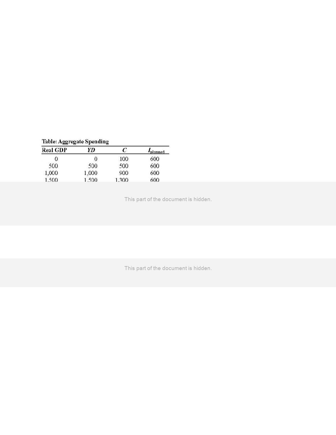
Use the following to answer questions 349-350:
Page 68
349.
(Table: Disposable Income and Spending) Use Table: Disposable Income and Spending.
Calculate the marginal propensity to consume (MPC). Use this MPC to compute the
spending multiplier.
350.
(Table: Disposable Income and Spending) Use Table: Disposable Income and Spending
Develop a linear equation of the consumption function. Use this consumption function
to forecast the amount of consumption spending that would occur if disposable income
were equal to $500.
Use the following to answer question 351:
351.
(Table: Aggregate Spending) Please refer to Table: Aggregate Spending. Suppose the
economy has no government spending and no foreign trade. With no taxes and transfers,
real GDP equals disposable income (YD). The data in the accompanying table show
consumption spending (C) and planned investment (IPlanned).
a. What is the marginal propensity to consume in this economy?
b. At what level of real GDP will the economy find its income–expenditure equilibrium?
352.
The multiplier process:
A)
explains how spending continues indefinitely with continuous rounds of spending.
B)
ends after one round of spending and with total spending limited to the initial
change in spending.
C)
occurs only when economies are in an expansion phase.
D)
is limited, with the total change in real GDP dependent upon the size of the
marginal propensity to consume.
Page 69
353.
The value of the multiplier will be smaller:
A)
the larger the value of the marginal propensity to save.
B)
the larger the value of the marginal propensity to consume.
C)
if the marginal propensity to consume equals the marginal propensity to save.
D)
if the marginal propensity to consume plus the marginal propensity to save equals
1.
354.
During the Great Depression:
A)
investment fell, but consumption increased.
B)
investment increased, but consumption decreased.
C)
both consumption and investment decreased.
D)
overall GDP rose.
355.
A factor that does NOT affect consumer spending is:
A)
current disposable income.
B)
wealth.
C)
past disposable income.
D)
expected disposable income.
356.
Two-thirds of total spending is usually attributed to:
A)
consumption.
B)
investment.
C)
government spending.
D)
net exports.
357.
The marginal propensity to save:
A)
is the change in consumer savings divided by the change in consumption.
B)
is the change in savings divided by the change in disposable income.
C)
equals MPC + 1.
D)
changes when the marginal propensity to consume is constant.
358.
Alice’s disposable income increases by $1,000, and she spends $600 of it. Assuming no
taxes, Alice’s:
A)
marginal propensity to save is 0.4 and she saves $400.
B)
MPC is 0.4 and she saves $400.
C)
marginal propensity to save is 0.4 and she saves $600.
D)
MPC is 0.6 and she consumes $400.
Page 70
359.
When Julie Ann’s disposable income is $10,000, she spends $10,000, and when her
disposable income is $15,000, her spending is $12,500. Julie Ann’s autonomous
consumption is _____ and her marginal propensity to consume is 0.5.
A)
$5,000
B)
$10,000
C)
$15,000
D)
$0
360.
The slope of the consumption function equals:
A)
1 – MPS.
B)
1 / (1 – MPS).
C)
1 – MPC.
D)
MPC / MPS.
361.
If housing values rise nationwide, there will be a(n):
A)
increase in consumer spending at any given level of disposable income.
B)
decrease in wealth as consumers spend more income on mortgage payments.
C)
decrease in overall aggregate expenditures.
D)
drop in investment spending.
362.
A decrease in consumer spending is likely to be caused by:
A)
expectation of an increase in personal income taxes.
B)
expectation of a decrease in personal income taxes.
C)
an increase in the multiplier.
D)
an increase in investment spending.
363.
When consumers receive more disposable income, their spending:
A)
will increase.
B)
will decrease.
C)
will stay the same, but their savings will decrease.
D)
and their savings will both decrease.
364.
The permanent income hypothesis suggests that consumer:
A)
spending depends on income people expect over the long term, rather than on
current income.
B)
spending is smoothed each month in response to changes in their current disposable
income.
C)
spending is made up of an autonomous amount and an amount dependent on
disposable income.
D)
savings depends on one’s lifetime income.
Page 71
365.
Vanessa tells people she is consuming more now and probably will continue to do so for
some time, but she believes her consumption will smooth out over her lifetime.
Vanessa’s consumption pattern mirrors the:
A)
multiplier hypothesis.
B)
life-cycle income hypothesis.
C)
relative income hypothesis.
D)
accelerator principle.
366.
Suppose the aggregate consumption function is given by C = 1,000 + 0.75YD, where C
is consumption and YD is disposable income. If disposable income increases by $100,
aggregate consumption will increase by _____ and autonomous consumption _____.
A)
$75; remains at $1,000
B)
$1000; remains at $75
C)
$100; increases by $100
D)
$175; increases by $100
367.
Suppose the aggregate consumption function is given by C = 1,000 + 0.75YD, where C
is consumption and YD is disposable income. If aggregate disposable income equals
$1,000, then aggregate consumption equals:
A)
$1,000.
B)
$1,750.
C)
$2,000.
D)
$1,075.
368.
Interest rates and planned investment spending:
A)
have a positive relationship.
B)
exhibit a negative relationship.
C)
have no relationship, since planned investment is fixed.
D)
have no relationship if the firm has retained earnings.
369.
A firm has enough retained earnings to finance an investment project. For this firm, the
market interest rate:
A)
is not relevant to the investment decision.
B)
indicates the opportunity cost of using retained earnings.
C)
will help to calculate the rate of return for the project.
D)
has no impact on the profitability of the investment project.