
Page 41
209.
The slope of the consumption function equals the slope of the:
A)
45-degree line.
B)
aggregate expenditure line.
C)
aggregate demand curve.
D)
short-run aggregate supply curve.
210.
Whenever real GDP exceeds planned aggregate expenditure, unplanned investment is
_____; whenever real GDP falls short of planned aggregate expenditure, unplanned
investment is _____.
A)
positive; negative
B)
negative; positive
C)
zero; positive
D)
zero; negative
211.
Whenever planned aggregate spending exceeds real GDP, unplanned inventory
investment is:
A)
negative.
B)
zero.
C)
positive.
D)
unpredictable.
212.
Whenever real GDP exceeds planned aggregate spending:
A)
firms reduce production, reducing real GDP.
B)
households increase consumption, increasing disposable income.
C)
firms increase production, increasing real GDP.
D)
households decrease consumption, decreasing disposable income.
213.
Income–expenditure equilibrium real GDP is the level of real GDP at which:
A)
the unemployment rate is zero.
B)
GDP equals planned aggregate spending.
C)
there is no savings.
D)
autonomous consumption equals planned inventory investment.
214.
Income–expenditure equilibrium occurs when:
A)
real GDP equals planned aggregate spending.
B)
real GDP equals actual aggregate spending.
C)
real GDP equals unplanned aggregate expenditure.
D)
consumption and investment are equal.
Page 42
215.
If real GDP is smaller than planned aggregate spending:
A)
unplanned inventory investment is positive.
B)
real GDP will fall.
C)
the economy is in equilibrium.
D)
unplanned inventory investment is negative.
216.
If real GDP is greater than planned aggregate spending:
A)
unplanned inventory investment is negative.
B)
real GDP will fall.
C)
the economy is in equilibrium.
D)
real GDP will rise.
217.
At the income–expenditure equilibrium, _____ is zero.
A)
investment net of depreciation
B)
planned investment
C)
unplanned inventory investment
D)
inventory investment
218.
Positive unplanned inventory investment leads to:
A)
prices increasing.
B)
production increasing.
C)
firms hiring more workers.
D)
production decreasing.
219.
An unplanned fall in inventories leads to:
A)
prices falling.
B)
production falling.
C)
production increasing.
D)
interest rates increasing.
220.
The Keynesian cross was developed by:
A)
John Maynard Keynes.
B)
Paul Samuelson.
C)
Adam Smith.
D)
Robert Heilbroner.
Page 43
221.
In an income–expenditure equilibrium:
A)
there are no inventories.
B)
there is no unplanned inventory investment.
C)
inventory investment equals consumption.
D)
there are no savings.
Use the following to answer questions 222-223:
222.
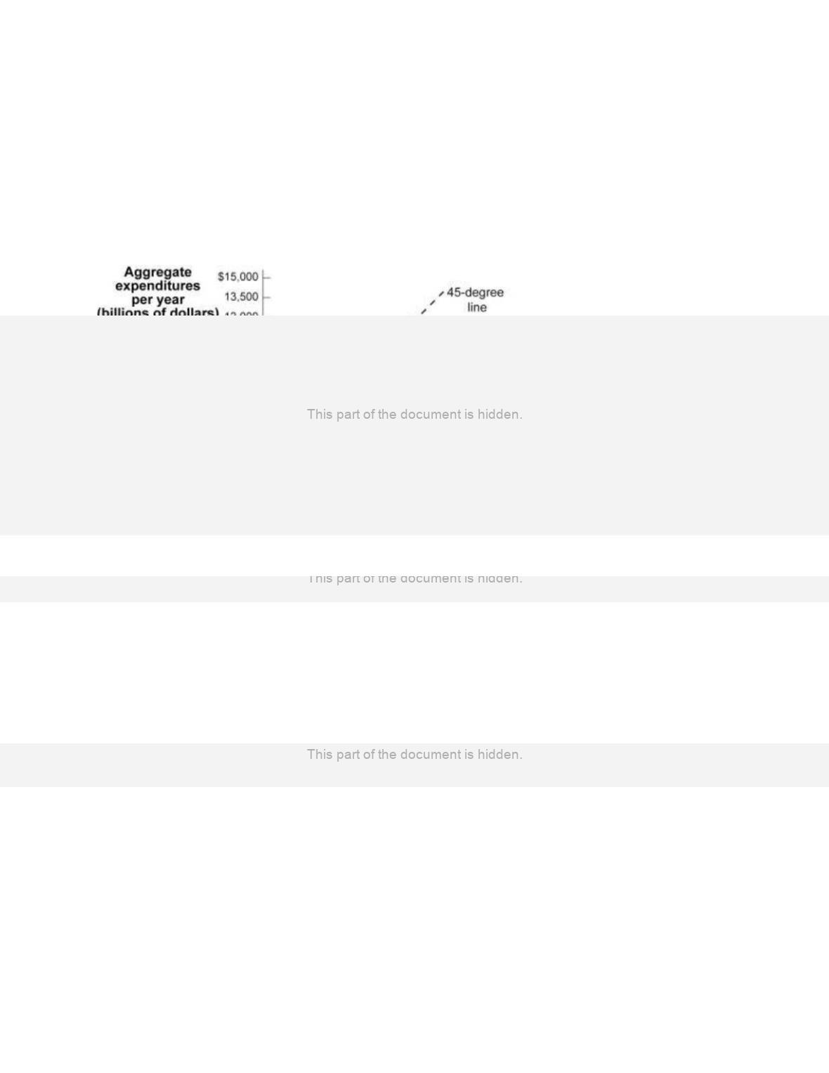
(Figure: Aggregate Expenditures and Real GDP) Use Figure: Aggregate Expenditures
and Real GDP. At a real GDP of $9,000 billion:
A)
planned investment is less than actual investment.
B)
planned investment equals actual investment.
C)
planned investment is greater than actual investment.
D)
there will be no unplanned investment.
223.
(Figure: Aggregate Expenditures and Real GDP) Use Figure: Aggregate Expenditures
and Real GDP. If the level of real GDP equals $9,000 billion and there are no changes
in the consumption function or in planned investment, then real GDP will _____in the
next period.
A)
rise
B)
remain unchanged
C)
fall
D)
fall, but only if there is an offsetting change in autonomous consumption

Page 44
224.
If aggregate expenditures are higher than real GDP:
A)
there are unplanned decreases in inventories.
B)
employment decreases.
C)
aggregate output decreases.
D)
actual real output is greater than equilibrium real output.
225.
If aggregate expenditures are lower than real GDP:
A)
there will be unplanned increases in inventories.
B)
employment increases.
C)
aggregate output increases.
D)
actual real output is less than equilibrium real output.
226.
If aggregate expenditures equal $800 billion and real GDP equals $600 billion:
A)
unplanned inventory accumulation equals $200 billion.
B)
unplanned inventory accumulation equals –$200 billion.
C)
consumption plus investment equals $200 billion.
D)
actual investment equals –$200 billion.
227.
If real GDP equals $700 billion and planned aggregate expenditures equal $400 billion:
A)
consumption plus planned investment equals $300 billion.
B)
actual investment equals –$300 billion.
C)
actual investment plus savings equals $300 billion.
D)
unplanned inventory accumulation equals $300 billion.
228.
If real GDP exceeds aggregate expenditures, the economy will:
A)
contract, reducing employment.
B)
expand, causing inflation.
C)
expand, increasing employment.
D)
neither contract nor expand, holding employment constant.
229.
If aggregate expenditures exceed real GDP, the economy will:
A)
expand, increasing employment.
B)
expand, reducing prices.
C)
contract, decreasing employment.
D)
neither expand nor contract, holding employment the same.
Page 45
Use the following to answer questions 230-231:
230.
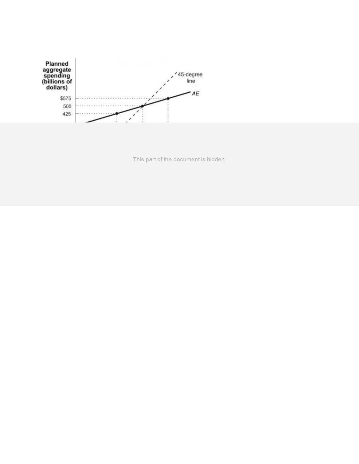
(Figure: Aggregate Expenditures I) Use Figure: Aggregate Expenditures I. The
equilibrium real GDP is:
A)
$500 billion.
B)
$300 billion.
C)
$700 billion.
D)
$625 billion.
231.
(Figure: Aggregate Expenditures I) Use Figure: Aggregate Expenditures I. When real
GDP is $700 billion, there will be a _____ in unplanned inventory investment.
A)
$125 million increase
B)
$125 million decline
C)
$200 million decline
D)
$200 million increase
232.
If real GDP is less than aggregate expenditure, then inventories will _____, and firms
will _____.
A)
increase; cut back on future production
B)
fall; decrease the prices of their products
C)
increase; lower their product prices
D)
fall; increase their future production

Page 46
233.
If real GDP is $1,000 billion and the aggregate expenditure is $850 billion, then the
change in inventories will be:
A)
–$150 million.
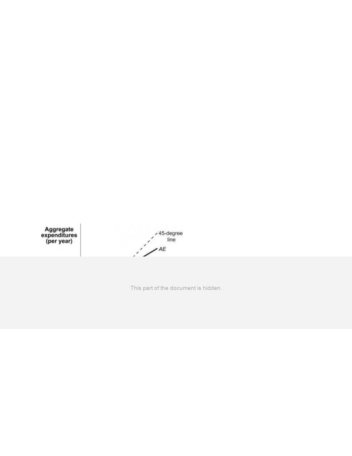
B)
$1,850 million.
C)
$150 million.
D)
–$1,850 million.
234.
When the economy is in income–expenditure equilibrium:
A)
exports equal imports.
B)
savings is less than investment spending.
C)
taxes equal transfer payments.
D)
real GDP equals planned aggregate spending.
235.
The Federal Reserve, the central bank of the United States, has been cutting the interest
rate to stimulate the recessionary economy. Interest rate cuts by the Federal Reserve are
supposed to:
A)
lower the savings rate in the economy and stop leakages.
B)
increase government spending on the economic infrastructure and thus increase
GDP through the multiplier process.
C)
increase cash holding by the general public, thus lowering their dependence on
credit.
D)
increase planned investment spending and thus increase GDP via the multiplier.
236.
If the slope of the aggregate expenditures curve is 0.8, the multiplier is:
A)
1.
B)
4.
C)
5.
D)
infinity.
237.
If the slope of the aggregate expenditures curve is 0.9, the multiplier is:
A)
1.
B)
4.
C)
5.
D)
10.
238.
If the slope of the aggregate expenditures curve is 0.75, the multiplier is:
A)
1.
B)
4.
C)
5.
D)
infinity.
Page 47
239.
The magnitude of the multiplier process that links planned aggregate spending to real
GDP is determined by the:
A)
marginal propensity to save.
B)
interest rate.
C)
level of autonomous consumption.
D)
level of planned investment spending.
240.
If planned aggregate spending rises by $10 billion and the marginal propensity to
consume is 0.75, then equilibrium real GDP changes by:
A)
$2.5 billion.
B)
$7.5 billion.
C)
$10 billion.
D)
$40 billion.
241.
If planned aggregate spending rises by $25 billion and the marginal propensity to
consume is 0.8, then equilibrium real GDP changes by:
A)
$25 billion.
B)
$125 billion.
C)
$200 billion.
D)
$250 billion.
242.
An autonomous increase in aggregate spending _____ real GDP by _____.
A)
reduces; that amount
B)
increases; that amount
C)
reduces; more than that amount
D)
increases; more than that amount
243.
The primary cause of the recession that ended in late 2001 was:
A)
a slump in business investment spending.
B)
too much investment spending by households, crowding out business investment
spending.
C)
an increase in income tax rates.
D)
a decrease in government spending.
244.
The recession began to wind down in late 2001 mainly because of an increase in:
A)
tax rates on capital gains.
B)
consumer spending on durable goods, especially automobiles.
C)
consumer spending on nondurables, especially gasoline and clothing.
D)
consumer savings.
Page 48
245.
In the last quarter of 2001, when consumer spending was ending the recession, GDP
growth was slow at first because:
A)
consumer savings also decreased.
B)
tax rates increased.
C)
inventories, which had built up during the recession, decreased.
D)
inventories of consumer goods increased.
246.
Real GDP is $8,000, autonomous consumption is $500, and planned investment
spending is $200. The marginal propensity to consume is 0.8. What is the consumption
function?
A)
C = 8,000 + 0.8* YD
B)
C = 8,700 + 0.2* YD
C)
C = 500 + 0.8* YD
D)
C = 1,700 + 0.2* YD
247.
Real GDP is $8,000, autonomous consumption is $500, and planned investment
spending is $200. The marginal propensity to consume is 0.8. How much is
consumption?
A)
$500
B)
$8,000
C)
$700
D)
$6,900
248.
Real GDP is $8,000, autonomous consumption is $500, and planned investment
spending is $200. The marginal propensity to consume is 0.8. How much is planned
aggregate spending?
A)
$7,100
B)
$6,400
C)
$8,000
D)
$700
249.
Real GDP is $8,000, autonomous consumption is $500, and planned investment
spending is $200. The marginal propensity to consume is 0.8. How much is unplanned
inventory investment?
A)
$1,100
B)
–$900
C)
$900
D)
0
Page 49
250.
Real GDP is $8,000, autonomous consumption is $500, and planned investment
spending is $200. The marginal propensity to consume is 0.8. Given this
income–expenditure equilibrium, firms will tend to:
A)
raise prices.
B)
hire more people.
C)
increase output.
D)
decrease output.
251.
Real GDP is $8,000, autonomous consumption is $500, and planned investment
spending is $200. The marginal propensity to consume is 0.8. If real GDP is $3,000,
planned aggregate spending is:
A)
$2,400.
B)
$2,900.
C)
$3,100.
D)
$3,000.
252.
Real GDP is $8,000, autonomous consumption is $500, and planned investment
spending is $200. The marginal propensity to consume is 0.8. If real GDP is $3,000,
how much is unplanned inventory investment?
A)
0
B)
$600
C)
$100
D)
–$100
253.
Real GDP is $8,000, autonomous consumption is $500, and planned investment
spending is $200. The marginal propensity to consume is 0.8. Income–expenditure
equilibrium is achieved when GDP is:
A)
$8,000.
B)
$7,000.
C)
$3,500.
D)
$700.
254.
Real GDP is $8,000, autonomous consumption is $500, and planned investment
spending is $200. The marginal propensity to consume is 0.8. The multiplier is:
A)
0.8.
B)
0.2.
C)
5.
D)
1.25.
Page 50
Use the following to answer questions 255-258:
255.
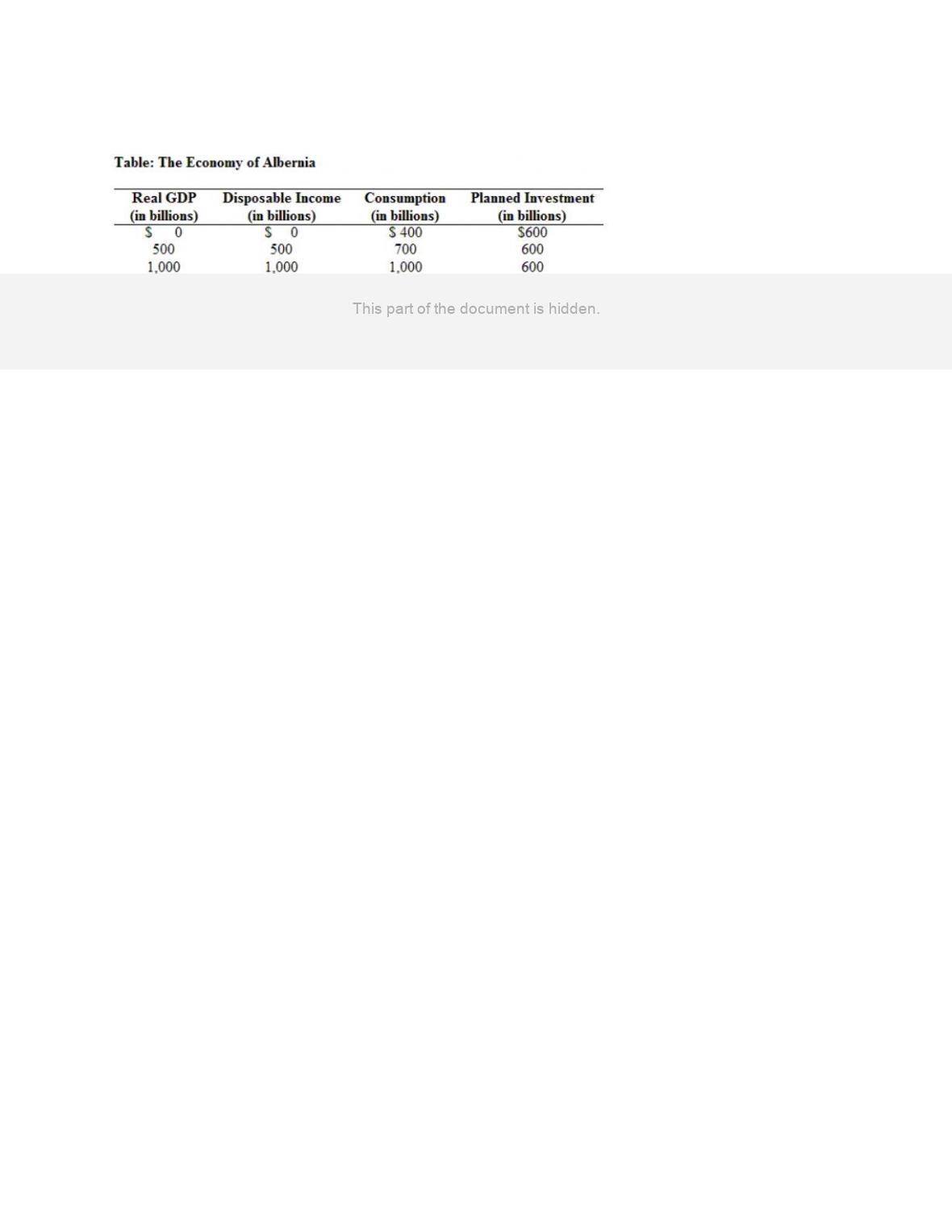
(Table: The Economy of Albernia) Use Table: The Economy of Albernia. What is the
consumption function for Albernia?
A)
C = 600 + 0.3* YD
B)
C = 600 + 0.75* YD
C)
C = 400 + 0.6* YD
D)
C = 400 + 0.75* YD
256.
(Table: The Economy of Albernia) Use Table: The Economy of Albernia. What is the
income–expenditure equilibrium real GDP?
A)
$1,000 billion
B)
$1,500 billion
C)
$2,000 billion
D)
$2,500 billion
257.
(Table: The Economy of Albernia) Use Table: The Economy of Albernia. If real GDP is
$1,500 billion, then the level of unplanned inventories is:
A)
$400 billion.
B)
–$400 billion.
C)
$600 billion.
D)
–$600 billion.
258.
(Table: The Economy of Albernia) Use Table: The Economy of Albernia. If real GDP is
$3,000 billion, then unplanned investment is:
A)
zero.
B)
$100 billion.
C)
$200 billion.
D)
$300 billion.
Page 51
Use the following to answer questions 259-262:
259.
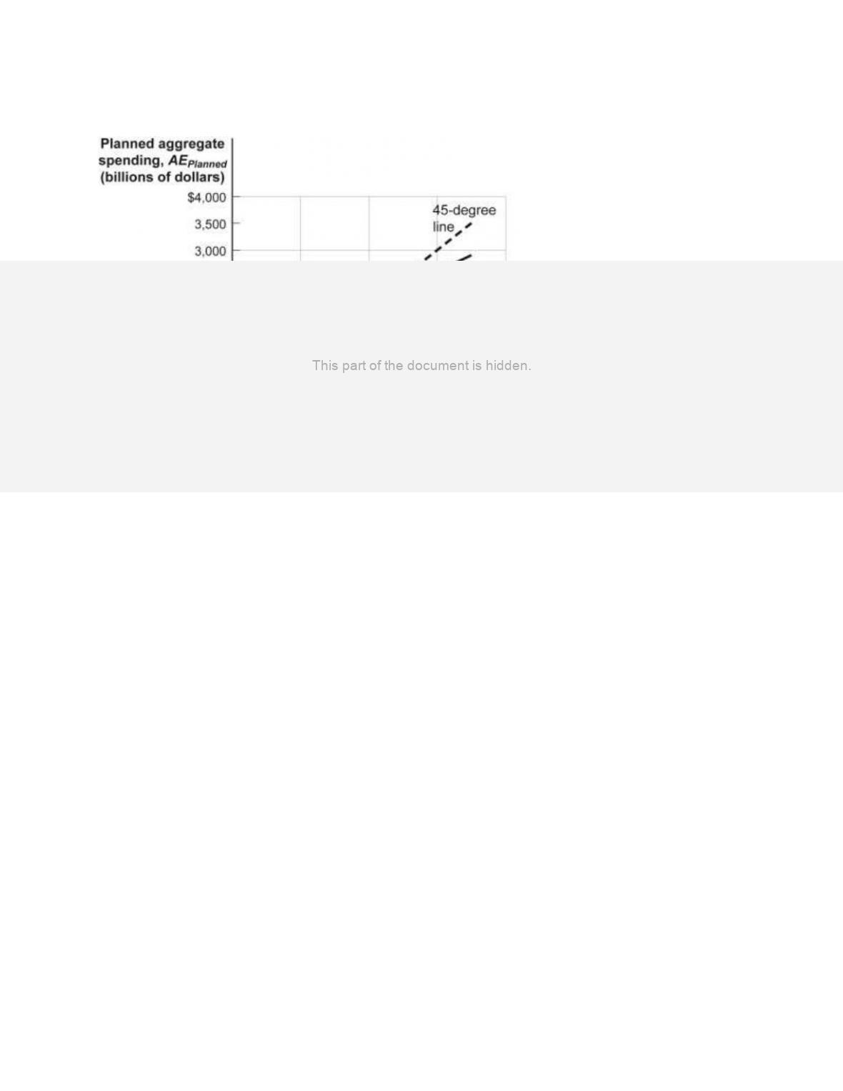
(Figure: Income–Expenditure Equilibrium) Use Table: Income–Expenditure
Equilibrium. If planned investment spending increases in this economy:
A)
aggregate expenditures curve will shift up, increasing the income–expenditure
equilibrium.
B)
aggregate expenditures curve will shift down, decreasing the income–expenditure
equilibrium.
C)
economy will move upward along the aggregate expenditures curve, increasing the
income–expenditure equilibrium.
D)
economy will move downward along the aggregate expenditures curve, decreasing
the income–expenditure equilibrium.
260.
(Figure: Income–Expenditure Equilibrium) Use Table: Income–Expenditure
Equilibrium. If investment spending decreases in this economy, then the:
A)
aggregate expenditures curve will shift up, increasing the income–expenditure
equilibrium.
B)
aggregate expenditures curve will shift down, decreasing the income–expenditure
equilibrium.
C)
economy will move upward along the aggregate expenditures curve, increasing the
income–expenditure equilibrium.
D)
economy will move downward along the aggregate expenditures curve, decreasing
the income–expenditure equilibrium.
Page 52
261.
(Figure: Income–Expenditure Equilibrium) Use Table: Income–Expenditure
Equilibrium. If planned investment spending increases autonomously by $100, real GDP
will:
A)
increase by $250.
B)
increase by $100.
C)
increase by $125.
D)
not change.
262.
(Figure: Income–Expenditure Equilibrium) Use Table: Income–Expenditure
Equilibrium. If planned investment spending increases by $100, the income–expenditure
equilibrium occurs at real GDP of:
A)
$8,100.
B)
$3,600.
C)
$2,250.
D)
$4,000.
Use the following to answer questions 263-265:
263.
(Table: Aggregate Spending) Use Table: Aggregate Spending. Suppose the economy
has no government spending and no foreign trade. With no taxes or transfers, real GDP
equals disposable income (YD). At what level of real GDP will the economy find its
income–expenditure equilibrium?
A)
$2,000
B)
$2,500
C)
$3,500
D)
$4,500
Page 53
264.
(Table: Aggregate Spending) Use Table: Aggregate Spending. Suppose the economy
has no government spending and no foreign trade. With no taxes or transfers, real GDP
equals disposable income (YD). If real GDP is $2,500, what is the level of unplanned
inventory investment?
A)
$200
B)
$0
C)
$2,700
D)
–$200
265.
(Table: Aggregate Spending) Use Table: Aggregate Spending. Suppose the economy
has no government spending and no foreign trade. With no taxes or transfers, real GDP
equals disposable income (YD). The income–expenditure equilibrium real GDP is found
at _____. If planned investment fell to $300, the new income–expenditure equilibrium
real GDP would fall to _____.
A)
$3,500; $2,500
B)
$3,500; $2,000
C)
$3,000; $1,500
D)
$4,000; $2,500
Use the following to answer questions 266-271:
266.
(Figure: Aggregate Expenditures Curve I) Use Figure: Aggregate Expenditures Curve I.
The equilibrium level of real GDP in the aggregate expenditures model shown in this
figure is:
A)
$800.
B)
$1,000.
C)
$1,600.
D)
$3,200.
Page 54
267.
(Figure: Aggregate Expenditures Curve I) Use Figure: Aggregate Expenditures Curve I.
The slope of the aggregate expenditures curve in this figure is:
A)
0.25.
B)
0.5.
C)
1.0.
D)
45 degrees.
268.
(Figure: Aggregate Expenditures Curve I) Use Figure: Aggregate Expenditures Curve I.
The multiplier in the aggregate expenditures model shown in this figure is:
A)
1.
B)
2.
C)
3.
D)
5.
269.
(Figure: Aggregate Expenditures Curve I) Use Figure: Aggregate Expenditures Curve I.
Suppose that the consumption function in this economy rises by $100. The result would
be a shift in the aggregate expenditures curve:
A)
upward by $100.
B)
upward by $200.
C)
upward by $100 times the multiplier.
D)
downward by $200.
270.
(Figure: Aggregate Expenditures Curve I) Use Figure: Aggregate Expenditures Curve I.
Suppose that the consumption function in this economy rises by $100. The result will be
a _____ increase in the equilibrium level of real GDP.
A)
$100
B)
$200
C)
$800
D)
$1,600
271.
(Figure: Aggregate Expenditures Curve I) Use Figure: Aggregate Expenditures Curve I.
Suppose that the government’s purchases of goods and services in this economy rise by
$100. Real GDP will:
A)
decrease by $100.
B)
increase by $200.
C)
increase by $800.
D)
decrease by $200.
Page 55
Use the following to answer questions 272-277:
272.
(Figure: Aggregate Expenditures Curve II) Use Table: Aggregate Expenditures Curve
II. The equilibrium level of real GDP in the aggregate expenditures model shown in this
figure is:
A)
$800.
B)
$1,000.
C)
$2,000.
D)
$4,000.
273.
(Figure: Aggregate Expenditures Curve II) Use Table: Aggregate Expenditures Curve
II. The slope of the aggregate expenditures curve is:
A)
0.25.
B)
0.5.
C)
0.6.
D)
45 degrees.
274.
(Figure: Aggregate Expenditures Curve II) Use Table: Aggregate Expenditures Curve
II. The multiplier is:
A)
1.0.
B)
2.0.
C)
2.5.
D)
5.0.
Page 56
275.
(Figure: Aggregate Expenditures Curve II) Use Table: Aggregate Expenditures Curve
II. Suppose that the consumption function in this figure rises by $100. The aggregate
expenditures curve would shift upward by:
A)
$100.
B)
$250.
C)
$100 times the multiplier.
D)
$150.
276.
(Figure: Aggregate Expenditures Curve II) Use Table: Aggregate Expenditures Curve
II. Suppose that the consumption function rises by $100. The equilibrium level of real
GDP would rise by:
A)
$100.
B)
$200.
C)
$250.
D)
$50.
277.
(Figure: Aggregate Expenditures Curve II) Use Table: Aggregate Expenditures Curve
II. Suppose that the consumption function in this economy rises by $200. Equilibrium
real GDP would rise by:
A)
$100.
B)
$200.
C)
$250.
D)
$500.
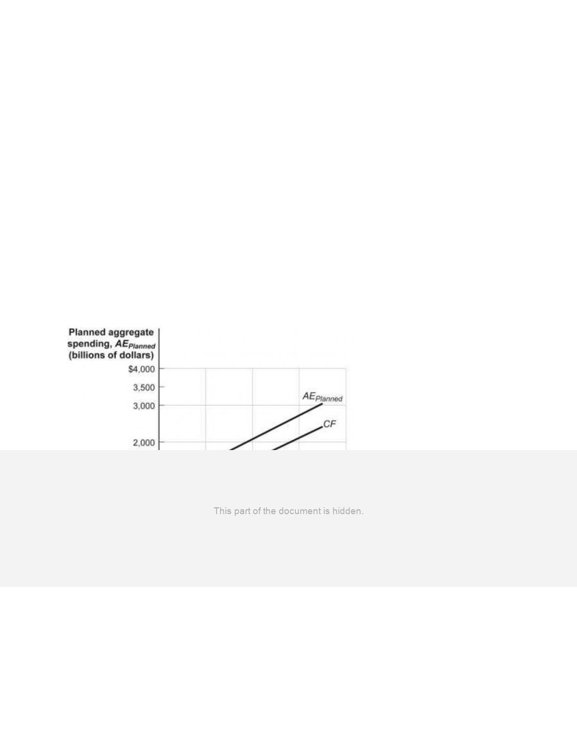
Use the following to answer questions 278-279:
Page 57
278.
(Figure: Aggregate Expenditures Curve III) Use Table: Aggregate Expenditures Curve
III. Suppose that the consumption function in this figure rises by $100. The aggregate
expenditures curve will shift upward by:
A)
$100.
B)
$400.
C)
$100 times the multiplier.
D)
$200 times the multiplier.
279.
(Figure: Aggregate Expenditures Curve III) Use Table: Aggregate Expenditures Curve
III. Suppose that the consumption function shifts upward by $100. Equilibrium real
GDP will rise by:
A)
$100.
B)
$400.
C)
$800.
D)
$3,200.
Use the following to answer questions 280-285:
Page 58
280.
(Figure: The Aggregate Consumption Function and Planned Aggregate Spending) Use
Figure: The Aggregate Consumption Function and Planned Aggregate Spending. If
current disposable income increases in this economy, then the:
A)
aggregate expenditures curve will shift up.
B)
aggregate expenditures curve will shift down.
C)
economy will move upward along the aggregate expenditures curve.
D)
economy will move downward along the aggregate expenditures curve.
281.
(Figure: The Aggregate Consumption Function and Planned Aggregate Spending) Use
Figure: The Aggregate Consumption Function and Planned Aggregate Spending. If
disposable income decreases, then the:
A)
aggregate expenditures curve will shift up.
B)
aggregate expenditures curve will shift down.
C)
economy will move upward along the aggregate expenditures curve.
D)
economy will move downward along the aggregate expenditures curve.
282.
(Figure: The Aggregate Consumption Function and Planned Aggregate Spending) Use
Figure: The Aggregate Consumption Function and Planned Aggregate Spending. If
expected disposable income increases, then the:
A)
aggregate expenditures curve will shift up.
B)
aggregate expenditures curve will shift down.
C)
economy will move upward along the aggregate expenditures curve.
D)
economy will move downward along the aggregate expenditures curve.
283.
(Figure: The Aggregate Consumption Function and Planned Aggregate Spending) Use
Figure: The Aggregate Consumption Function and Planned Aggregate Spending. If
expected disposable income decreases in this economy, then the:
A)
aggregate expenditures curve will shift up.
B)
aggregate expenditures curve will shift down.
C)
economy will move upward along the aggregate expenditures curve.
D)
economy will move downward along the aggregate expenditures curve.
284.
(Figure: The Aggregate Consumption Function and Planned Aggregate Spending) Use
Figure: The Aggregate Consumption Function and Planned Aggregate Spending. If
aggregate wealth increases, the:
A)
aggregate expenditures curve will shift up.
B)
aggregate expenditures curve will shift down.
C)
economy will move upward along the aggregate expenditures curve.
D)
economy will move downward along the aggregate expenditures curve.
Page 59
285.
(Figure: The Aggregate Consumption Function and Planned Aggregate Spending) Use
Figure: The Aggregate Consumption Function and Planned Aggregate Spending. If
aggregate wealth decreases, then the:
A)
aggregate expenditures curve will shift up.
B)
aggregate expenditures curve will shift down.
C)
economy will move upward along the aggregate expenditures curve.
D)
economy will move downward along the aggregate expenditures curve.
286.
The digital revolution led to a decline in Finnish paper exports.
A)
True
B)
False
287.
Finland’s real GDP per capita grew rapidly in 2008 due to Nokia’s ability to innovate
and stay ahead of its competition.
A)
True
B)
False
288.
From 2010 to 2012, North Dakota’s economy grew at an annual growth rate of 17%,
more than 5 times the growth of the U.S. economy as a whole, due to rapid growth in its
biotechnology sector.
A)
True
B)
False
289.
From 2010 to 2012, North Dakota’s economy grew at an annual growth rate of 17%,
more than 5 times the growth of the U.S. economy as a whole due to the mining of
shale.
A)
True
B)
False
290.
The marginal propensity to consume is the increase in consumer spending when
disposable income increases by $1.
A)
True
B)
False
291.
The marginal propensity to save is the increase in household savings when investment
spending increases by $1.
A)
True
B)
False
Page 60
292.
In a simple, closed economy (no government or foreign sector), any disposable income
that is not consumed is saved.
A)
True
B)
False
293.
In a simple, closed economy (no government or foreign sector), if disposable income
increases by $500 and $450 is consumed, $950 is saved.
A)
True
B)
False
294.
In a simple, closed economy (no government or foreign sector), if disposable income
increases by $500 and $450 is consumed, $50 is saved.
A)
True
B)
False
295.
A $200 million increase in investment spending will increase real GDP by exactly $200
million.
A)
True
B)
False
296.
A $200 million increase in investment spending will increase real GDP by more than
$200 million.
A)
True
B)
False
297.
A $300 million decrease in investment spending will increase real GDP by more than
$300 million.
A)
True
B)
False
298.
A $600 million decrease in investment spending will decrease real GDP by more than
$600 million.
A)
True
B)
False