38-101
Copyright © 2018 McGraw-Hill Education. All rights reserved. No reproduction or distribution without the prior
written consent of McGraw-Hill Education.
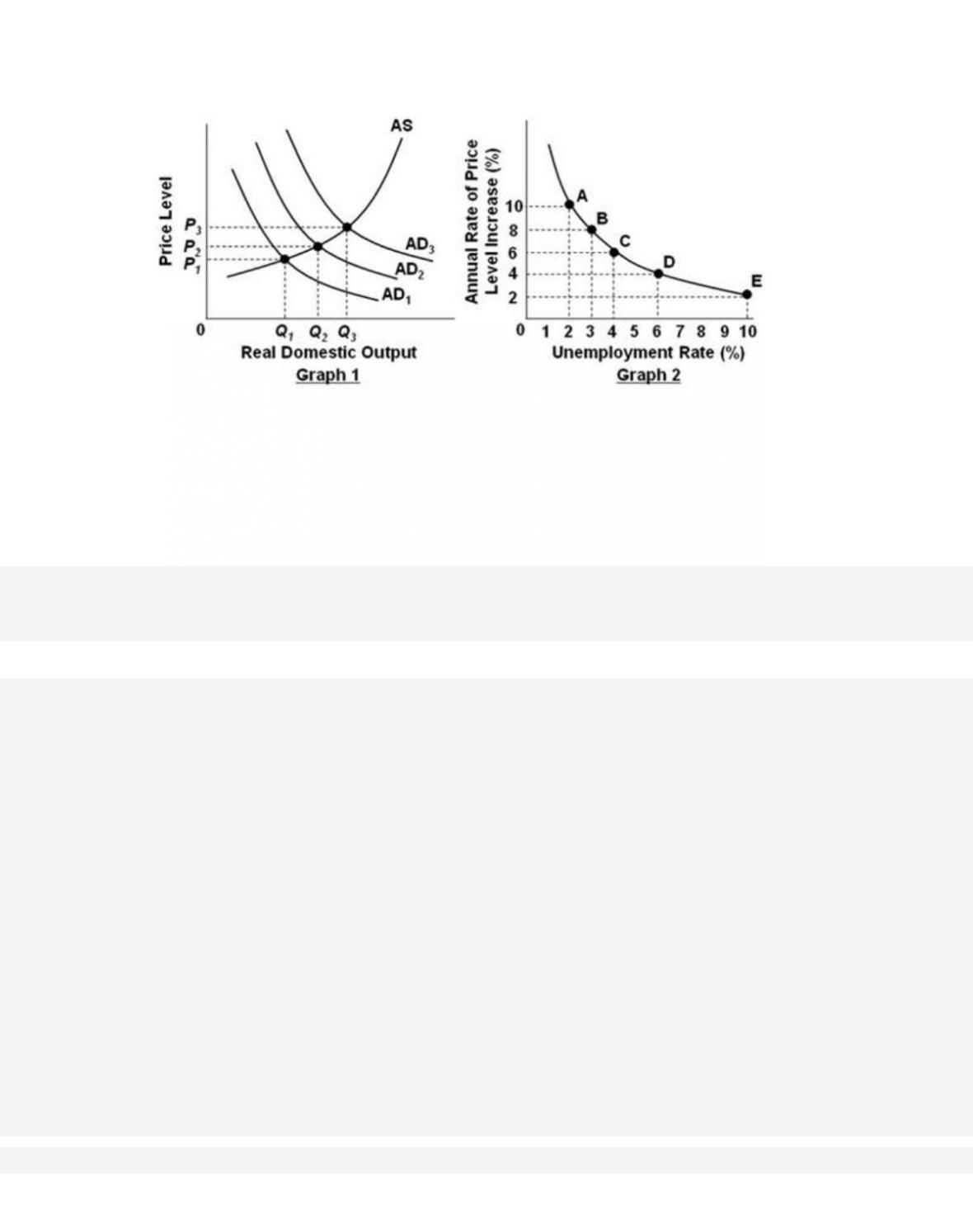
A.
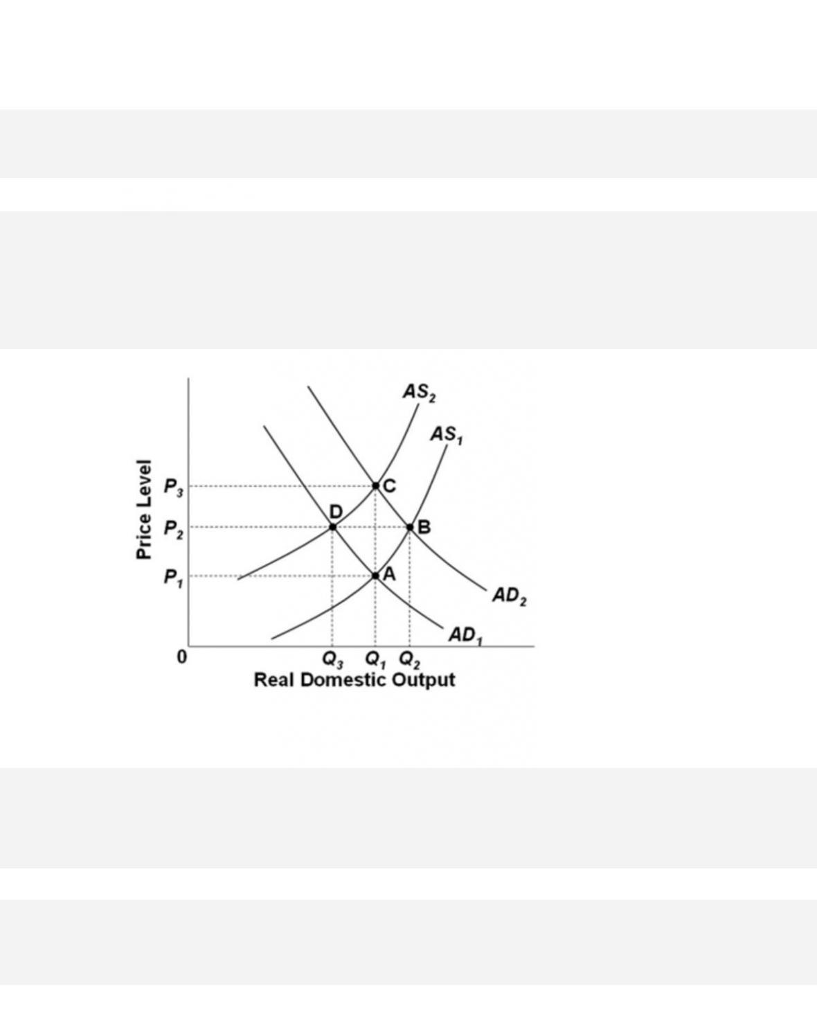
P1, and output will be at Q1.
B.
P3, and output will be at Q1.
C.
P2, and output will be at Q2.
D.
P3, and output will be at Q3.
164.
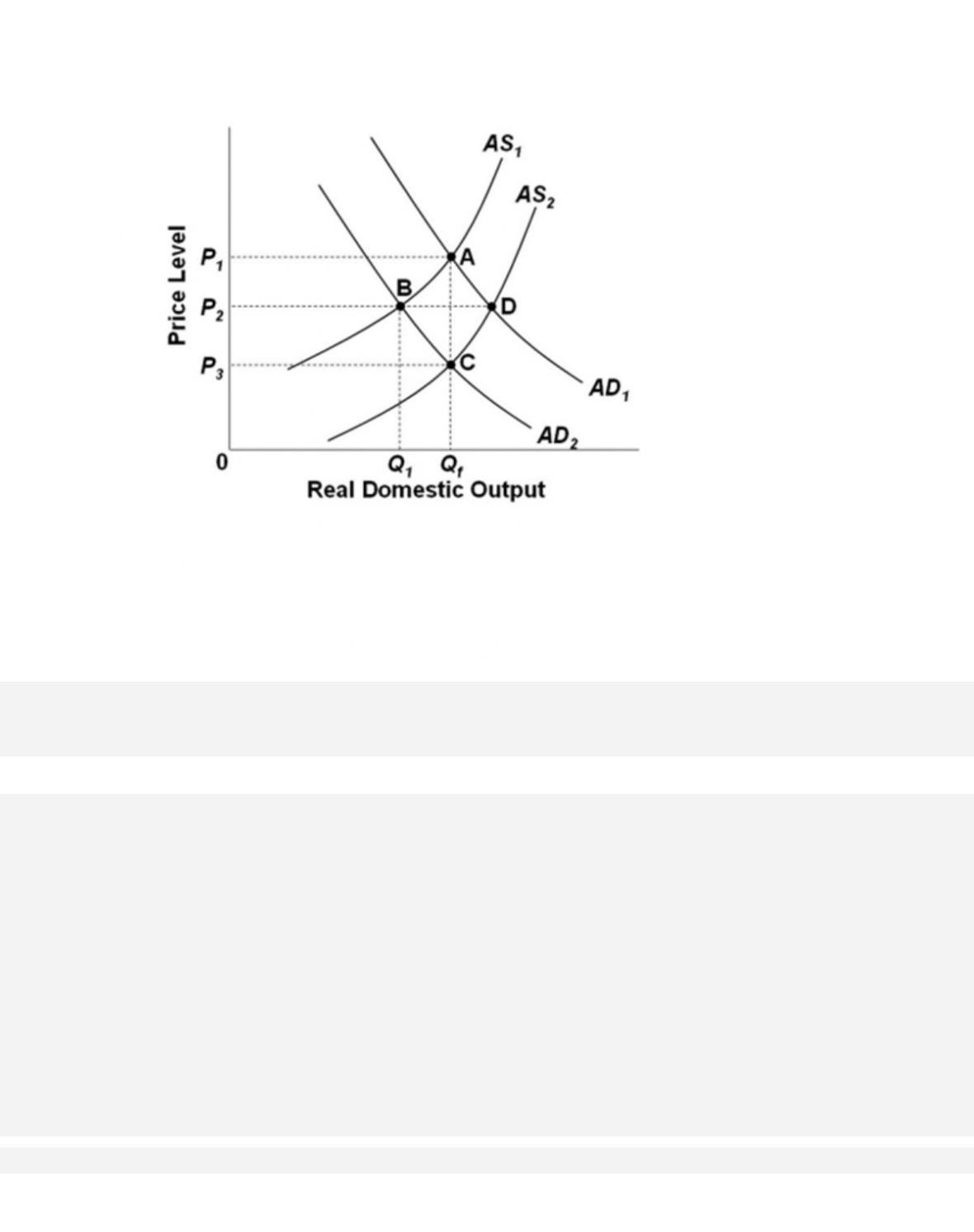
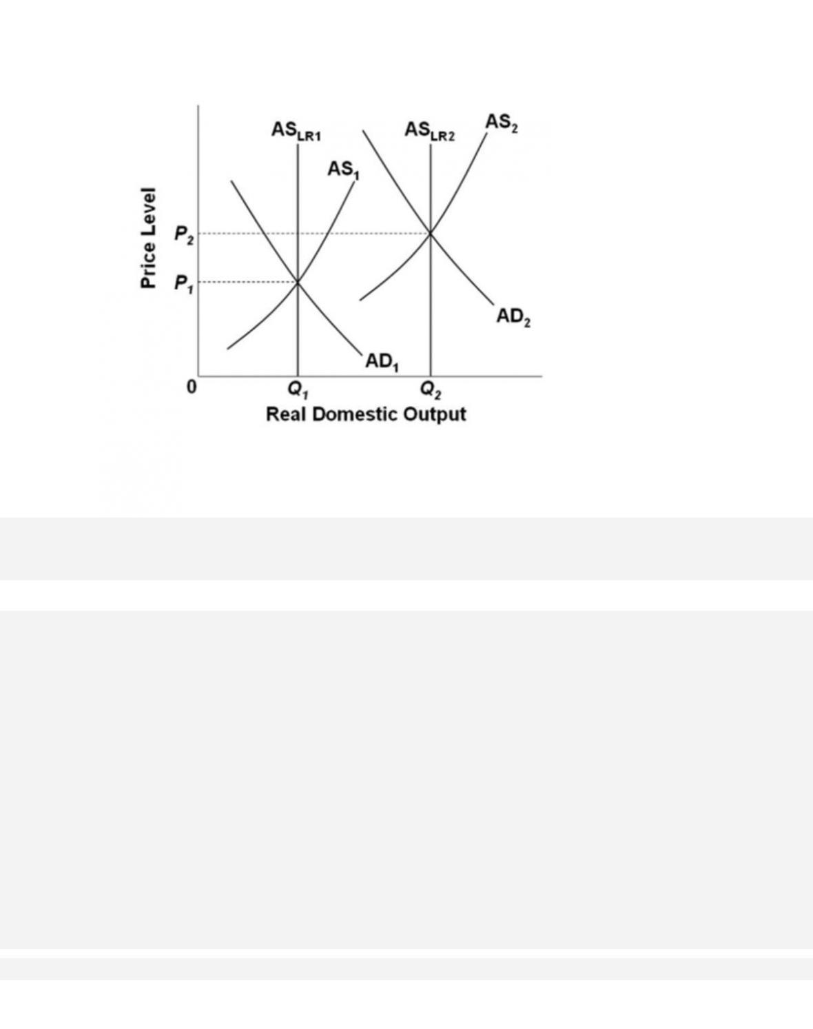
Refer to the graph. Assume that the economy is initially at full-employment equilibrium at
38-102
Copyright © 2018 McGraw-Hill Education. All rights reserved. No reproduction or distribution without the prior
written consent of McGraw-Hill Education.
Difficu l t y : 02 Medium
Learning Objective: 38-02 Discuss how to apply the “extended” (short-run/long-run) AD–AS
model to inflation, recessions, and economic growth.
Test Bank: II
Topic: Applying the Extended AD–AS Model
Type: Graph
165.
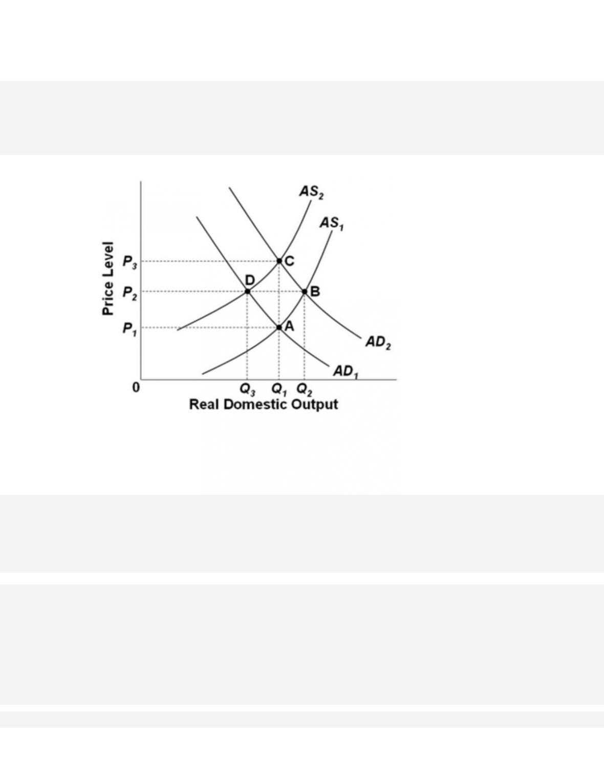
Refer to the graph. Assume that the economy is initially at full-employment equilibrium at
point A. If there is cost-push inflation in this
economy and the government pursues an
expansionary fiscal policy, then in the long run the
166.
Refer to the graph. Assume that the economy is initially at equilibrium at point A. If there is
a recession in the economy because AD1
shifts to AD2, and wages and prices are flexible,
then in the long run the price level will be
167.
Refer to the graph. If Qf is potential GDP and wages and prices are flexible, then the long-
run aggregate supply curve will be
168.
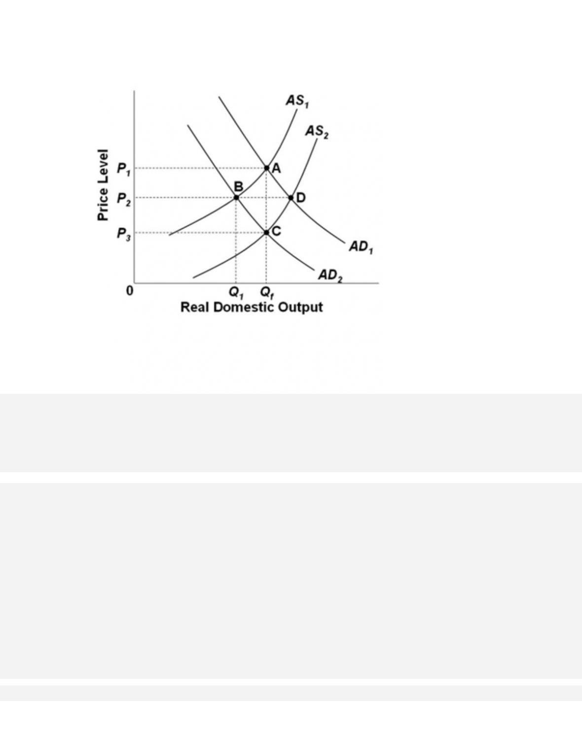
Refer to the graph. Assume that the economy is initially at equilibrium at point C and that the
government has adopted a hands-off policy
approach. If demand-pull inflation occurs, then
the final long-run equilibrium point will be point ; while if cost-push inflation occurs
(starting at point C), then the final long-run equilibrium point will be point .

169.
Refer to the graph. Economic growth driven by productivity and technology would be
illustrated as a shift of
170.
Refer to the graph. An expansion of the economy‘s production possibilities can, by itself
171.
Refer to the graph. Ongoing inflation would occur if the Fed
172.
The traditional Phillips Curve shows the

38-109
Copyright © 2018 McGraw-Hill Education. All rights reserved. No reproduction or distribution without the prior
written consent of McGraw-Hill Education.
D.
inverse correlation between the short-run and long-run aggregate supply.
173.
The traditional Phillips Curve showing a trade-off between inflation and
unemployment is based on having a stable
174.
If the economy is operating in the intermediate range of the aggregate supply curve, then
the greater the rate of growth of aggregate
demand, the
38-110
Copyright © 2018 McGraw-Hill Education. All rights reserved. No reproduction or distribution without the prior
written consent of McGraw-Hill Education.
Learning Objective: 38-03 Explain the short-run trade-off between inflation and unemployment
(the Phillips Curve).
Test Bank: II
Topic: The Inflation-Unemployment Relationship
175.
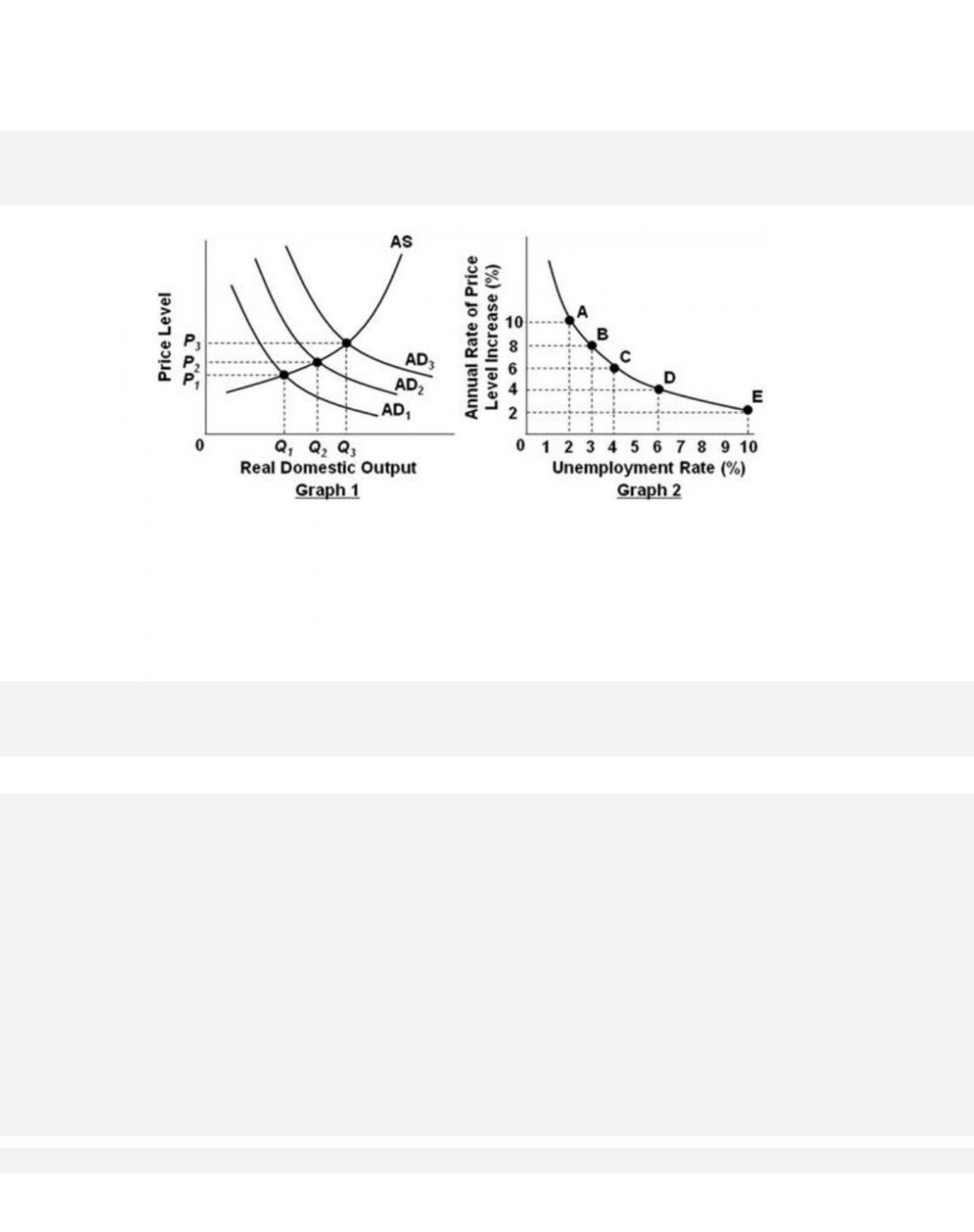
Refer to the graphs. Assume that the economy is initially at equilibrium where AD2 and AS
intersect in Graph 1, and also assume that the
economy is initially at point C in Graph 2. A
movement from point C to point B in graph 2 would most likely be associated, in graph 1,
with a shift of
176.
Refer to the graphs. Assume that the economy is initially at equilibrium where AD2 and AS
intersect in Graph 1, and also assume that the
economy is initially at point C in Graph 2. If
the government implements a contractionary or restrictive policy, it would make the
economy in graph 2
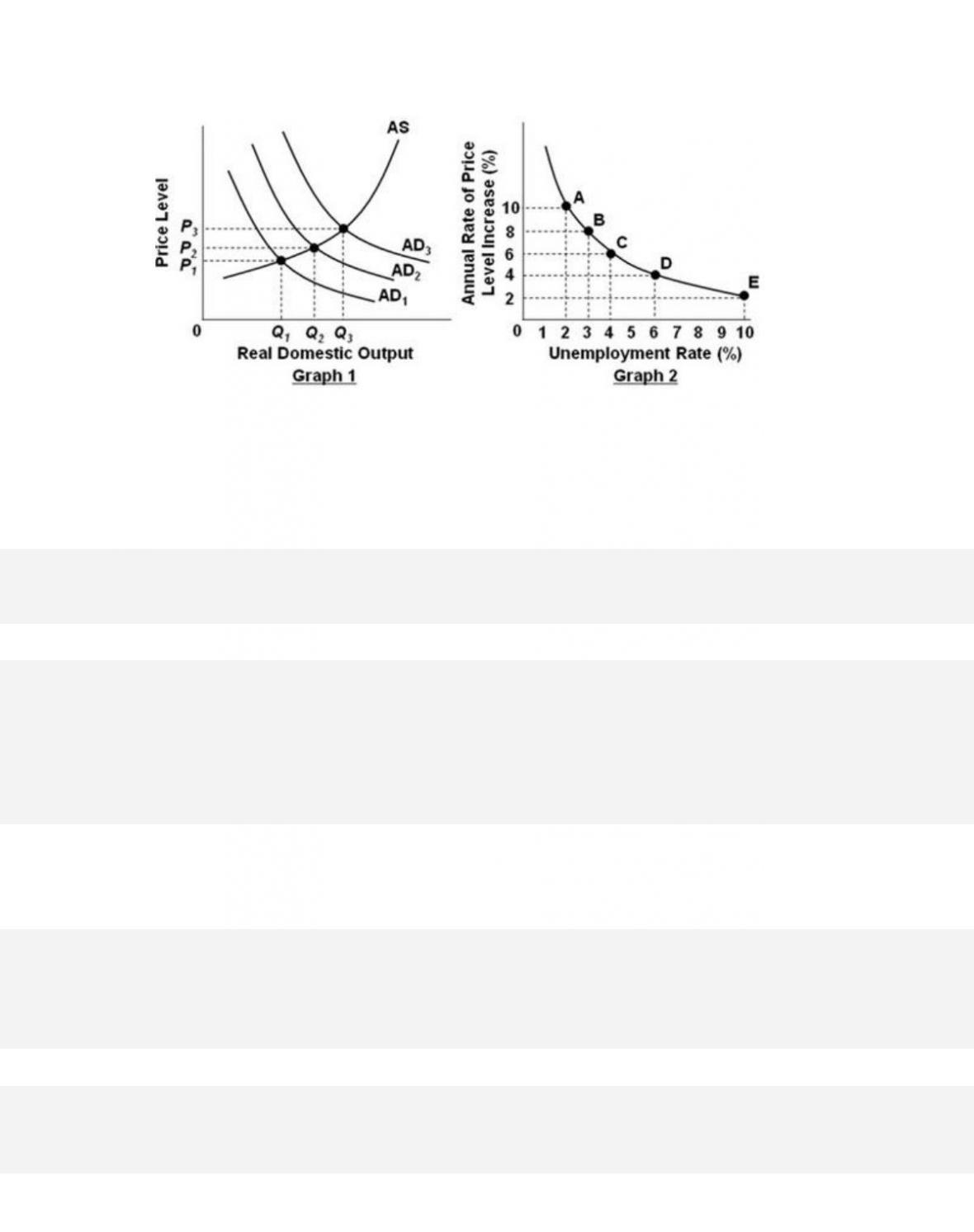
177.
Refer to the graphs. Assume that the economy starts out at point D in Graph 2, whereas full
employment would be attained at point C. The
Phillips curve shown suggests that full
employment
178.
Given a Phillips Curve with stable and predictable inflation and unemployment rate
trade-offs, it appears that

38-113
Copyright © 2018 McGraw-Hill Education. All rights reserved. No reproduction or distribution without the prior
written consent of McGraw-Hill Education.
Access i b i lity: Keyboard Navigation
Blooms: Understand
Difficu l t y : 02 Medium
Learning Objective: 38-03 Explain the short-run trade-off between inflation and unemployment
(the Phillips Curve).
Test Bank: II
Topic: The Inflation-Unemployment Relationship
179.
The inflation and unemployment data for the 1970s suggest that the aggregate-supply
shocks of that period caused the
180.
Adverse aggregate-supply shocks or stagflation would cause a
181.
A rightward shift of the Phillips Curve suggests that

182.
Stagflation can be described as a
183.
Which event probably contributed to the stagflation of the 1970s?

38-115
Copyright © 2018 McGraw-Hill Education. All rights reserved. No reproduction or distribution without the prior
written consent of McGraw-Hill Education.
Test Bank: II
Topic: The Inflation-Unemployment Relationship
184.
Adverse aggregate supply shocks would result in
185.
A potential cause of stagflation is
186.
Which factor contributed to the demise of stagflation during the 1982–1989 period?

38-116
Copyright © 2018 McGraw-Hill Education. All rights reserved. No reproduction or distribution without the prior
written consent of McGraw-Hill Education.
Blooms: Understand
Difficu l t y : 02 Medium
Learning Objective: 38-03 Explain the short-run trade-off between inflation and unemployment
(the Phillips Curve).
Test Bank: II
Topic: The Inflation-Unemployment Relationship
187.
Stagflation’s demise during the 1980s resulted in a
188.
In the period 2011 through 2015, as the economy slowly mended, the economy
experienced an ongoing pattern of falling inflation
coinciding with falling unemployment.
This suggests a
189.
The misery index is a measure of national economic discomfort that adds together a
nation‘s

38-117
Copyright © 2018 McGraw-Hill Education. All rights reserved. No reproduction or distribution without the prior
written consent of McGraw-Hill Education.
A.
saving and investment.
B.
budget deficit and public debt.
C.
unemployment rate and inflation rate.
D. level of taxation with the amount of government spending.
190.
Consider the following national data: tax revenues as a percentage of GDP: 25 percent;
government spending as a percentage of GDP: 31
percent; unemployment rate: 9 percent;
inflation rate: 6 percent. What is the misery index for this nation?
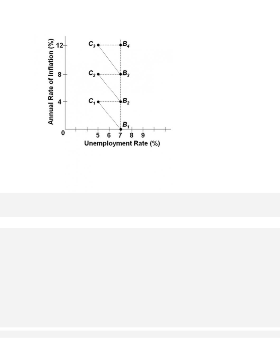
191.
Refer to the graph. Assume the economy is at the initial position of B2. An increase in
aggregate demand with no corresponding change in
inflation expectations and wage rates
will tend to
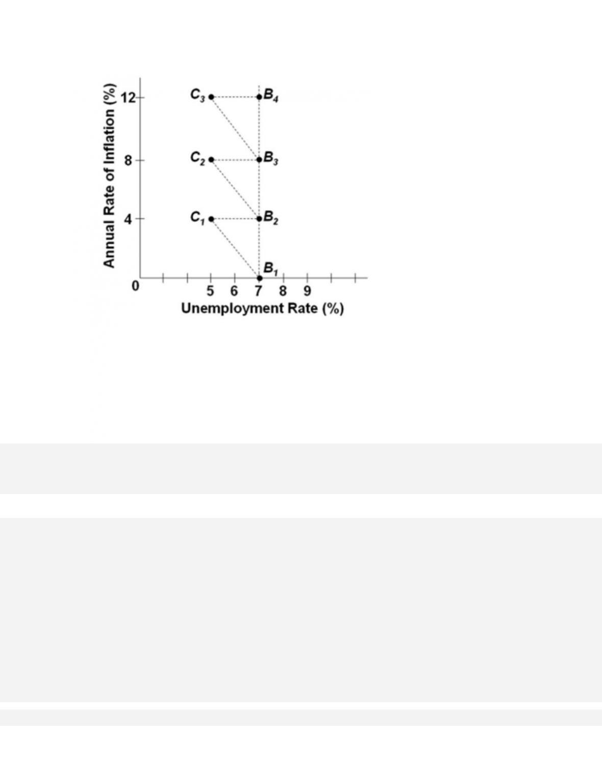
192.
Refer to the graph. Assume the economy is at the initial position of B2. An increase in
aggregate demand with a corresponding adjustment
in inflation expectations and wages
will tend to
193.
Refer to the graph. Assume the economy is at the initial position of B2. It is possible for the
government to reduce the unemployment rate
and move the economy to C2 if