
38–81
Refer to the accompanying economic data for a hypothetical economy. The given data
indicate that the economy has entered a period of
demand-pull inflation.
128.
Year
Average
Hourly Wage
Rates
Index of
Industrial
Production
Unemployment
Rate
Price
Level
Index
Rate of Increase in
Productivity
1997
$6.40
197
5.5%
130
3.0%
1998
6.72
199
5.8
133
2.9
1999
7.24
196
7.2
139
3.1
2000
8.02
192
8.3
147
2.8
Refer to the accompanying economic data for a hypothetical economy. It would be the
appropriate stabilization policy to raise interest
rates, raise taxes, and reduce government
expenditures.
129.
Year
Average
Hourly Wage
Index of
Industrial
Unemployment
Rate
Price
Level
Rate of Increase in
Productivity

Rates
Production
Index
1997
$6.40
197
5.5%
130
3.0%
1998
6.72
199
5.8
133
2.9
1999
7.24
196
7.2
139
3.1
2000
8.02
192
8.3
147
2.8
Refer to the accompanying economic data for a hypothetical economy. There is evidence that
cost-push inflationary pressure is present in
this economy.
130.
Year
Average
Hourly Wage
Rates
Index of
Industrial
Production
Unemployment
Rate
Price
Level
Index
Rate of Increase in
Productivity
1997
$6.40
197
5.5%
130
3.0%
1998
6.72
199
5.8
133
2.9
1999
7.24
196
7.2
139
3.1
2000
8.02
192
8.3
147
2.8
Refer to the accompanying economic data for a hypothetical economy. This economy has
encountered stagflation.

Type: Table
Multiple Choice Questions
131.
In the short run, the price level is assumed to be
132.
In the short run, nominal wages and other input prices are assumed to be
133.
The economy enters the long-run once

38–84
Copyright © 2018 McGraw-Hill Education. All rights reserved. No reproduction or distribution without the prior
written consent of McGraw-Hill Education.
C.
sufficient time has elapsed for wage contracts to expire and nominal wages to adjust to
output-price changes.
D. sufficient time has elapsed for real GDP to increase and unemployment to decrease as a
consequence
134.
Assume that initially your nominal wage was $16 an hour and the price index was 100.
If the price level increases to 105, then your
135.
In the short run, if the price level increases, then nominal wages

38–85
Copyright © 2018 McGraw-Hill Education. All rights reserved. No reproduction or distribution without the prior
written consent of McGraw-Hill Education.
Test Bank: II
Topic: From Short Run to Long Run
136.
The short-run aggregate supply curve illustrates the idea that if the price level falls,
firms will experience
137.
In the long run, if the price level increases, then nominal wages and other input prices
will
138.
In the long run, if the price level decreases, then the economy‘s output level will
38–86
Copyright © 2018 McGraw-Hill Education. All rights reserved. No reproduction or distribution without the prior
written consent of McGraw-Hill Education.
AACSB: Knowledge Application
Access i b i lity: Keyboard Navigation
Blooms: Understand
Difficu l t y : 02 Medium
Learning Objective: 38-01 Explain the relationship between short-run aggregate supply and
long-run aggregate supply.
Test Bank: II
Topic: From Short Run to Long Run
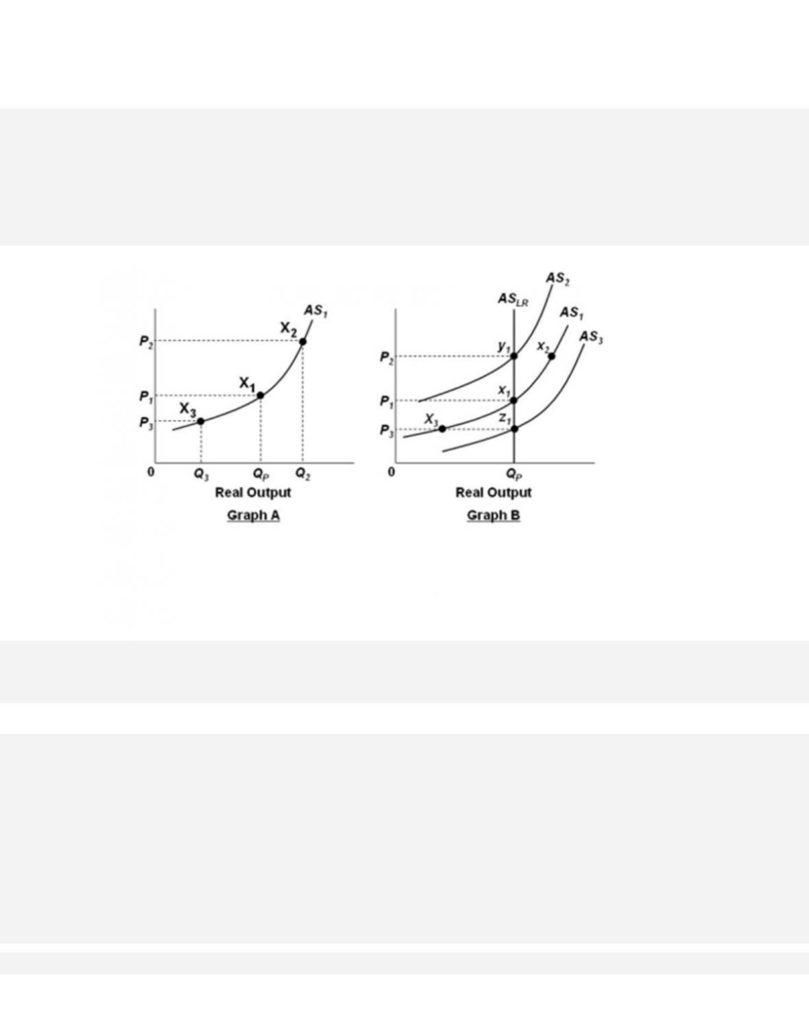
139.
In the accompanying graphs, QP refers to the economy‘s potential output level. Graph A is
constructed on the basic assumption that

140.
In the accompanying graphs, QP refers to the economy’s potential output level. In Graph A,
an increase in the price level from P1 to P2
will cause

141.
In the accompanying graphs, QP refers to the economy‘s potential output level. In Graph A, a
decrease in the price level from P1 to P3
will lead to
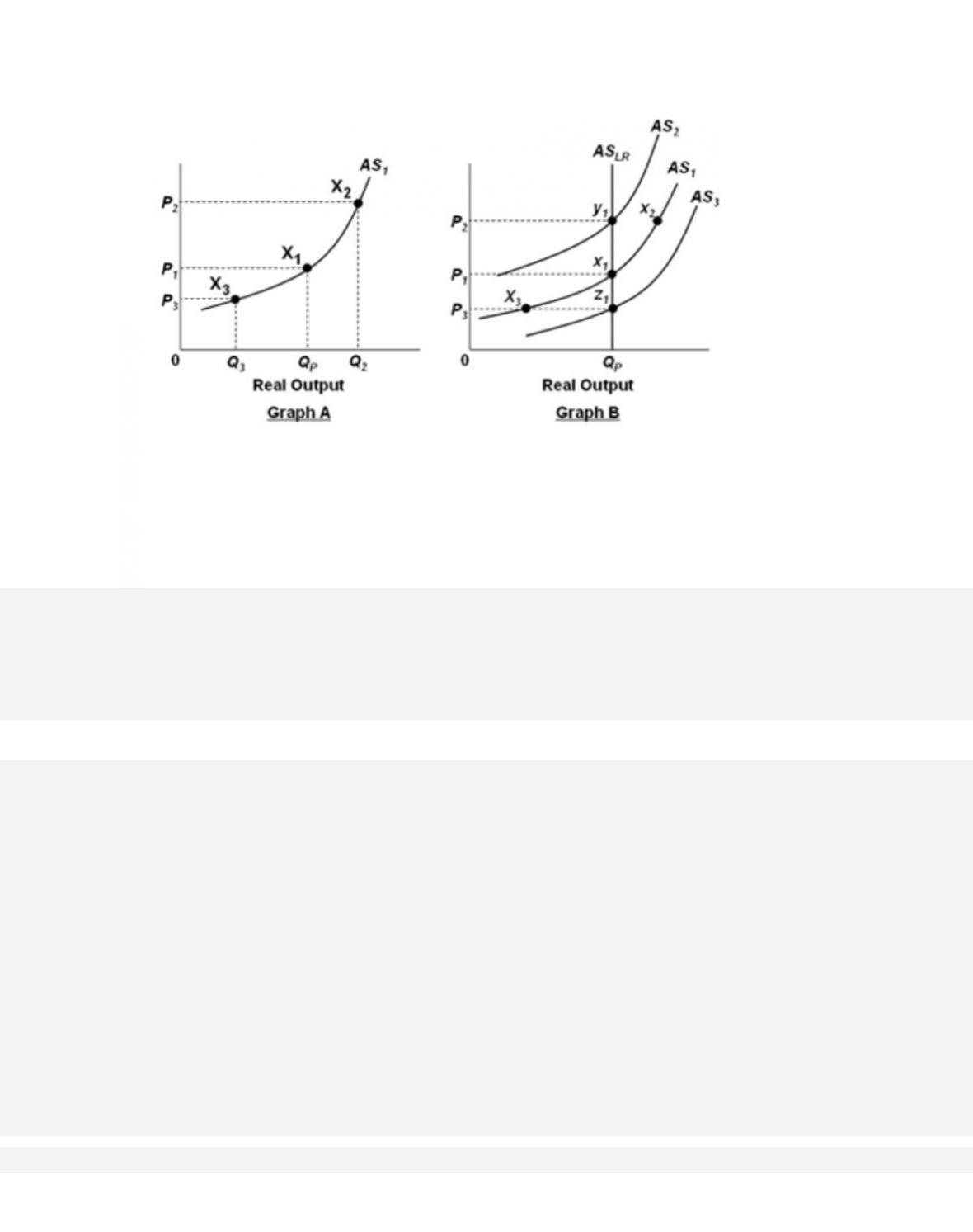
142.
In the accompanying graphs, QP refers to the economy‘s potential output level. In Graph B,
assume that the economy is initially in
equilibrium at point x1 but then there is an increase
in the price level from P1 to P2. In the long run, this change will lead to

143.
In the accompanying graphs, QP refers to the economy‘s potential output level. In Graph B,
assume that the economy is initially in
equilibrium at point x1 but then there is an increase
in the price level from P1 to P2. This change will lead to
144.
The short-run aggregate supply curve

38–91
Copyright © 2018 McGraw-Hill Education. All rights reserved. No reproduction or distribution without the prior
written consent of McGraw-Hill Education.
AACSB: Knowledge Application
Access i b i lity: Keyboard Navigation
Blooms: Understand
Difficu l t y : 02 Medium
Learning Objective: 38-01 Explain the relationship between short-run aggregate supply and
long-run aggregate supply.
Test Bank: II
Topic: From Short Run to Long Run
145.
The short-run aggregate supply curve intersects the long-run aggregate supply curve at
146.
Equilibrium in the long run occurs when
147.
Inflation in the short run is most likely to result from a(n)

38–92
Copyright © 2018 McGraw-Hill Education. All rights reserved. No reproduction or distribution without the prior
written consent of McGraw-Hill Education.
B.
decrease in aggregate demand or aggregate supply.
C.
increase in aggregate demand or a decrease in aggregate supply.
D. decrease in aggregate demand or an increase in aggregate supply.
148.
Demand-pull inflation in the short run raises the price level and
149.
In the long run, demand-pull inflation

38–93
Copyright © 2018 McGraw-Hill Education. All rights reserved. No reproduction or distribution without the prior
written consent of McGraw-Hill Education.
Test Bank: II
Topic: Applying the Extended AD–AS Model
150.
In the long run, demand-pull inflation leads to
151.
With demand-pull inflation in the extended AD–AS model, there is
152.
In the short-run, demand-pull inflation increases

38–94
Copyright © 2018 McGraw-Hill Education. All rights reserved. No reproduction or distribution without the prior
written consent of McGraw-Hill Education.
D.
real output and the price level, but in the long-run only the price level.
153.
In the cost-push model of inflation, increases in nominal-wage rates that exceed
increases in the productivity of labor
154.
If the government uses expansionary monetary or fiscal policies to counter the output
effects of cost-push inflation, then the economy is
likely to experience

155.
If the government adopts a hands-off approach to cost-push inflation in the economy,
then in the short run there is likely to be
156.
If cost-push inflation occurs and the government adopts a hands–off policy approach,
then, according to the simple extended AD–AS
model, in the long run the economy will
157.
What will occur in the short run if there is cost-push inflation and the government
adopts a hands-off approach to it?
38–96
Copyright © 2018 McGraw-Hill Education. All rights reserved. No reproduction or distribution without the prior
written consent of McGraw-Hill Education.
Access i b i lity: Keyboard Navigation
Blooms: Understand
Difficu l t y : 02 Medium
Learning Objective: 38–02 Discuss how to apply the “extended” (short-run/long-run) AD–AS
model to inflation, recessions, and economic growth.
Test Bank: II
Topic: Applying the Extended AD–AS Model
158.
If prices and wages are flexible, a decrease in aggregate demand will in the long run
cause only a(n)
159.
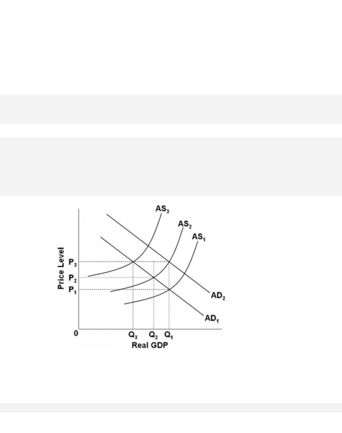
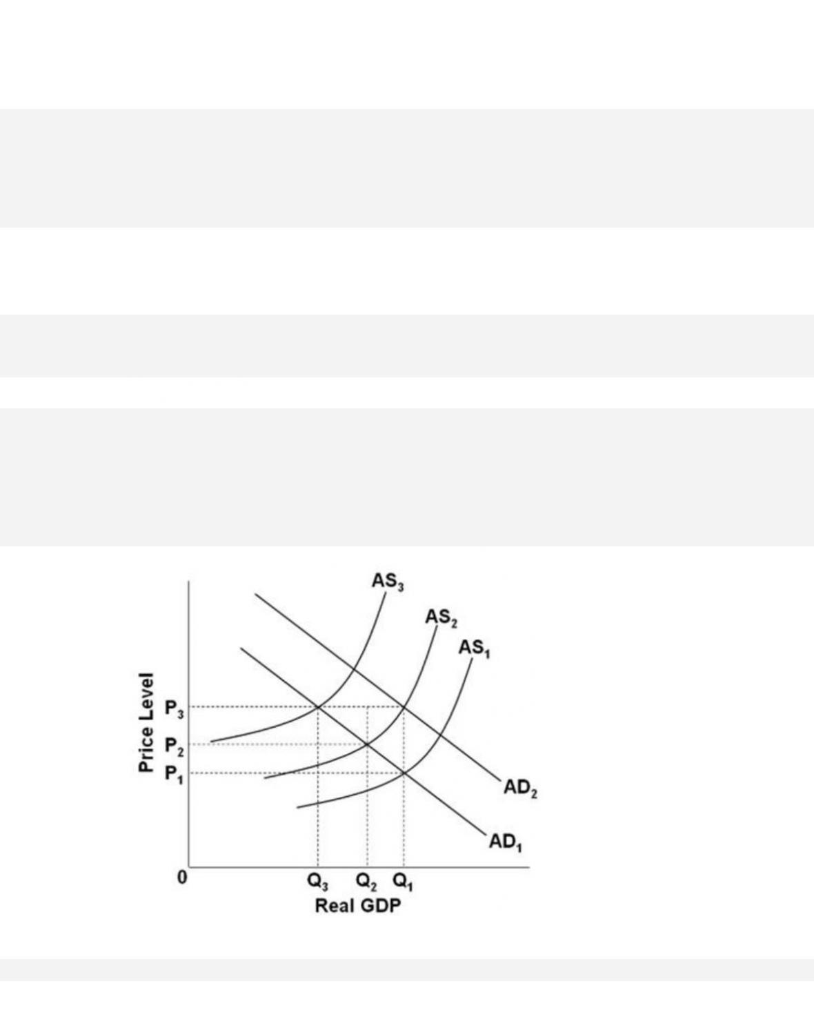
38–97
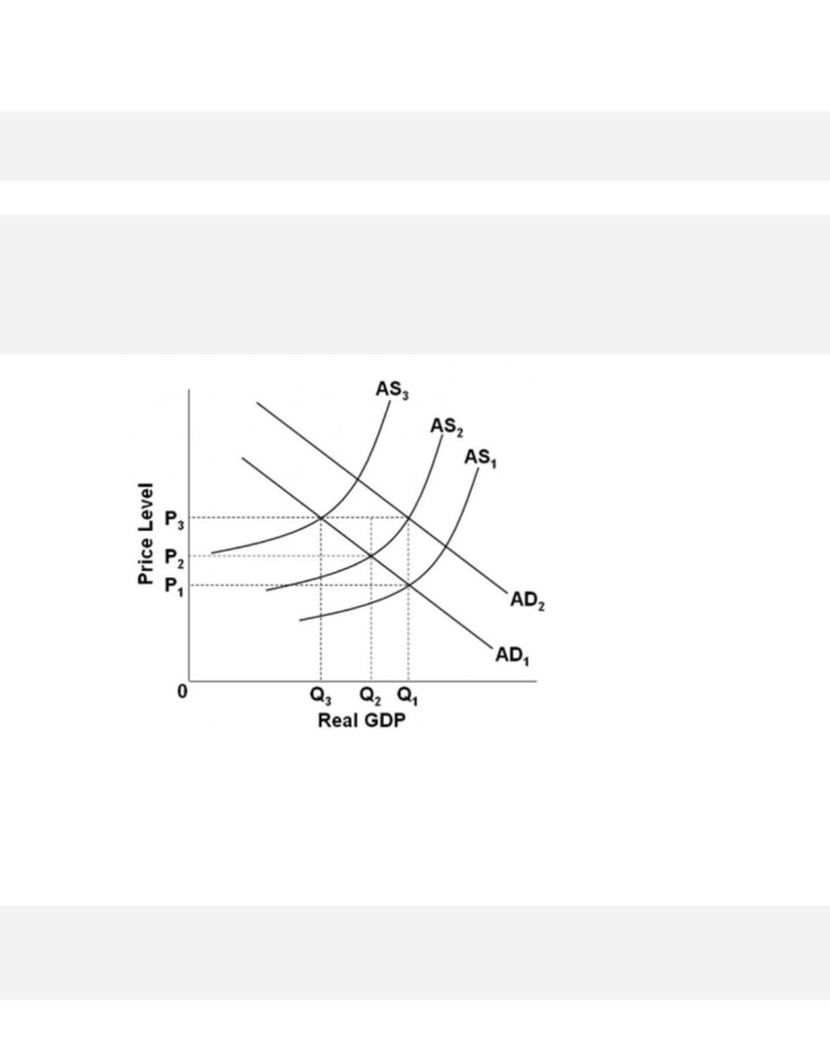
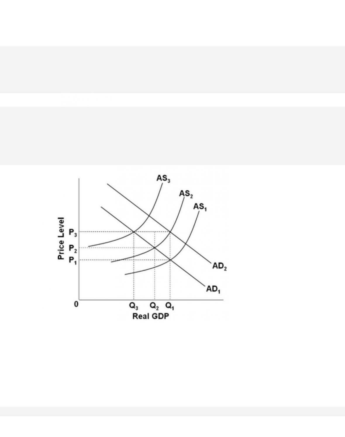
Refer to the graph. Suppose that the economy is at an initial equilibrium where the AD1 and
AS1 curves intersect. Demand-pull inflation
in the short run can best be represented as a
shift of
160.
Refer to the graph. Suppose that the economy is at an initial equilibrium where the AD1 and
AS1 curves intersect. Demand-pull inflation
in the long run can best be illustrated as a shift
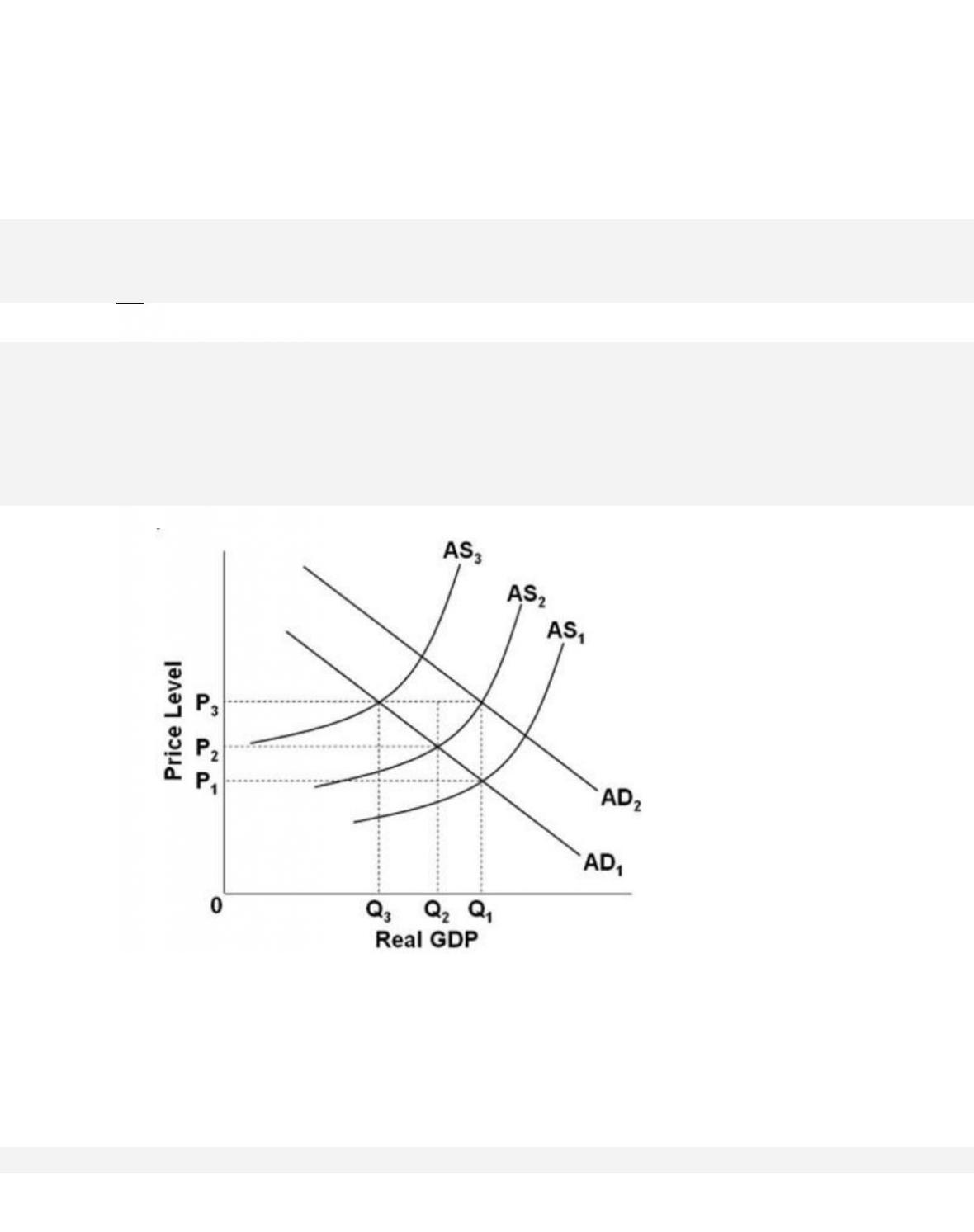
38–98
of
161.
Refer to the graph. Stagflation in the short run is best represented as resulting from a shift of
38–99
Copyright © 2018 McGraw-Hill Education. All rights reserved. No reproduction or distribution without the prior
written consent of McGraw-Hill Education.
A.
AD1 to AD2, given a stable AS1 curve.
B.
AD2 to AD1, given a stable AS1 curve.
C.
AS1 to AS2, given a stable AD1 curve.
D. AS2 to AS1, given a stable AD1 curve.
162.
Refer to the graph. Suppose that the economy is at an initial equilibrium where the AD1 and
AS1 curves intersect. If cost-push inflation
occurs and the government subsequently
implements expansionary policy, then the effect of such policy is to shift
38-100
Copyright © 2018 McGraw-Hill Education. All rights reserved. No reproduction or distribution without the prior
written consent of McGraw-Hill Education.
B.
AS1 to AS2, which increases the price level from P1 to P2 and decreases real output
from Q1 to Q2.
C.
AD1 to AD2, which increases the price level from P2 to P3 and increases real output
from Q2 to Q1.
D. AS2 to AS3, which increases the price level from P2 to P3 and decreases real output
from Q2 to Q3.
163.
Refer to the graph. Suppose that the economy is at an initial equilibrium where the AD1 and
AS1 curves intersect. If cost-push inflation
occurs and the government adopts a hands-off
policy approach, then in the long run the price level will be at