31-121
Copyright © 2018 McGraw-Hill Education. All rights reserved. No reproduction or distribution without the prior
written consent of McGraw-Hill Education.
FA LSE
229.
If government decreases its purchases by $20 billion and the MPC is 0.8, equilibrium
GDP will decrease by $100 billion.
230.
If the MPC is 0.9, a $20 billion increase in a lump-sum tax will reduce GDP by $200
billion.
231.
A recessionary expenditure gap in a mixed open economy can be measured as the extent
to which aggregate expenditures (Ca + Ig + Xn + G) fall short of real GDP at the full–
employment level of real GDP.
232.
The recessionary expenditure gap is the amount by which the equilibrium GDP and the
full-employment GDP differ.
Multiple Choice Questions
233.
The most basic premise of the aggregate expenditures model is that
D. the unemployment level in the economy is inversely related to the inflation rate.
234.
One basic assumption of the aggregate expenditures model is that
A.
the economy is operating at full employment.
235.
John Maynard Keynes developed the aggregate expenditures model in order to understand
the
A.
Second World War.
236.
In the aggregate-expenditures model, the average price level is
A.
measured along the horizontal axis.
31-124
Copyright © 2018 McGraw-Hill Education. All rights reserved. No reproduction or distribution without the prior
written consent of McGraw-Hill Education.
Learning Objective: 31–01 Explain how sticky prices relate to the aggregate expenditures
model.
Test Bank: II
To p i c :
Assumptions and Simplifications
237.
In a private closed economy, the two components of aggregate expenditures are
A.
consumption and government spending.
238.
In the aggregate expenditures model, the consumption schedule is shown to be
A.
directly related to real interest rates.
239.
The investment schedule shows the
A.
inverse relationship between the expected rate of return and the quantity of investment
demanded.
31-125
Copyright © 2018 McGraw-Hill Education. All rights reserved. No reproduction or distribution without the prior
written consent of McGraw-Hill Education.
D. rate of interest that business firms must pay when they make investments in capital goods.
240.
The difference between the investment demand curve and the investment schedule is that
the former shows
A.
a direct relationship between investment and interest rate, while the latter shows no
correlation between investment and income.
241.
Which of the following is graphed as a horizontal line across levels of real GDP in the
aggregate expenditures model?
A.
the saving schedule
31-126
Copyright © 2018 McGraw-Hill Education. All rights reserved. No reproduction or distribution without the prior
written consent of McGraw-Hill Education.
Learning Objective: 31-02 Explain how an economys investment schedule is derived from the
investment demand curve and an interest rate.
Test Bank: II
To p i c :
Consumption and Investment Schedules
242.
In the aggregate expenditures model, which of the following variables is assumed to be
independent of real GDP?
A.
profit
243.
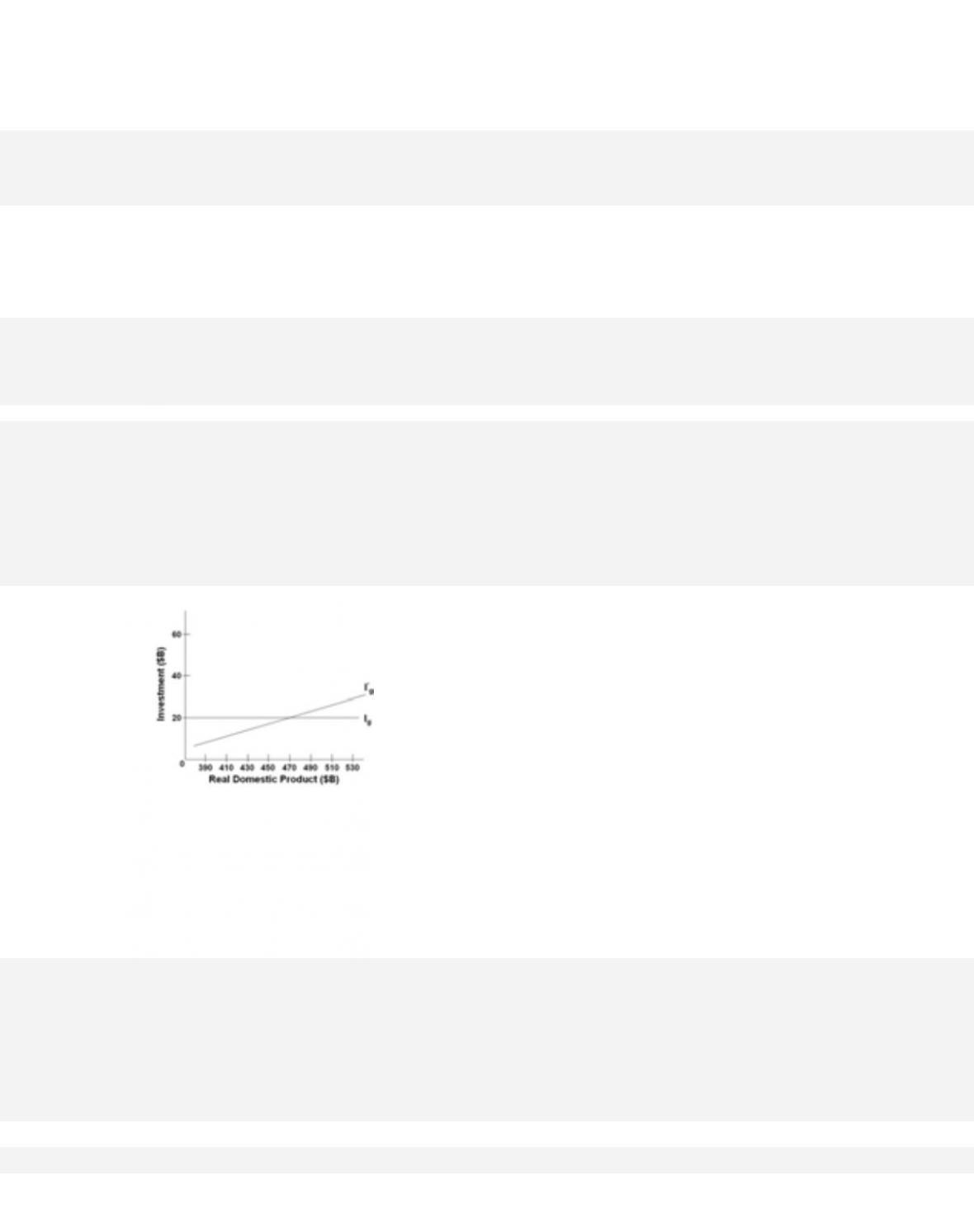
The accompanying graph indicates that
A. I’g is an investment schedule that assumes that the investment plans of business are
independent of the current level of income, whereas Ig does not.
31-127
Copyright © 2018 McGraw-Hill Education. All rights reserved. No reproduction or distribution without the prior
written consent of McGraw-Hill Education.
AACSB: Knowledge Application
Blooms: Understand
Di ff i cu l ty :
02 Medium
Learning Objective: 31-02 Explain how an economys investment schedule is derived from the
investment demand curve and an interest rate.
Test Bank: II
To p i c :
Consumption and Investment Schedules
244. A rightward shift of the investment demand curve will
A.
shift the investment schedule downward.
245. If the real interest rate falls, then the
D. consumption schedule will shift downward.
246. If the stock of available capital in the economy is running too low, then the

31-128
Copyright © 2018 McGraw-Hill Education. All rights reserved. No reproduction or distribution without the prior
written consent of McGraw-Hill Education.
C. consumption schedule will shift upward.
D. consumption schedule will shift downward.
247. If the expected rate of return on investment decreases, then most likely the
A.
investment schedule will shift upward.
248. In a private closed economy, the equilibrium condition for the economy is
C. AE = C + Ig + G = GDP.
D. C + Ig + G + NX = GDP.
31-129
Copyright © 2018 McGraw-Hill Education. All rights reserved. No reproduction or distribution without the prior
written consent of McGraw-Hill Education.
To p i c :
Equilibrium GDP: C Ig = GDP
249. When aggregate expenditure is greater than GDP, then there will be an
A.
unplanned increase in inventories and GDP will increase.
250. In a private closed economy, there will be an unplanned increase in inventories when
A.
aggregate expenditures exceed GDP.
251.
Domestic Output or Income (GDP=DI)
Consumption
$540
$540
560
555
580
570
31-130
600
585
620
600
640
615
660
630
The table gives data for a private (no government) closed economy. All figures are in billions
of dollars. If planned investment is $25 billion, then aggregate expenditures at the income level
of $560 billion will be
A. $565 billion.
252.
Domestic Output or Income (GDP=DI)
Consumption
$540
$540
560
555
580
570
600
585
620
600
640
615
660
630
The table gives data for a private (no government) closed economy. All figures are in billions
of dollars. If planned investment is $25 billion, the equilibrium level of GDP will be
A.
$600 billion.
253.
Domestic Output or Income (GDP=DI)
Consumption
$540
$540
560
555
580
570
600
585
620
600
640
615
660
630
The table gives data for a private (no government) closed economy. All figures are in billions
of dollars. If planned investment is $15 billion, then at the $560 billion level of output, there
will be an
A.
unplanned increase in inventories of $5 billion.
31-132
Copyright © 2018 McGraw-Hill Education. All rights reserved. No reproduction or distribution without the prior
written consent of McGraw-Hill Education.
goods produced equals the total quantity of goods purchased.
Test Bank: II
To p i c :
Equilibrium GDP: C Ig = GDP
254.
Domestic Output or Income (GDP=DI)
Consumption
$540
$540
560
555
580
570
600
585
620
600
640
615
660
630
The table gives data for a private (no government) closed economy. All figures are in billions
of dollars. If planned investment is $18 billion, then at the $660 billion level of disposable
income, there will be an
D. unplanned decrease in inventories of $30 billion.
255.
Domestic Output or Income (GDP=DI)
Consumption
$240
$244
250
250
260
256
270
262
280
268
31-133
290
274
300
280
310
286
320
292
Refer to the table. All figures are in billions of dollars. When there is no investment in this
private closed economy, the equilibrium level of GDP will be
A. $240 billion.
256.
Domestic Output or Income (GDP=DI)
Consumption
$240
$244
250
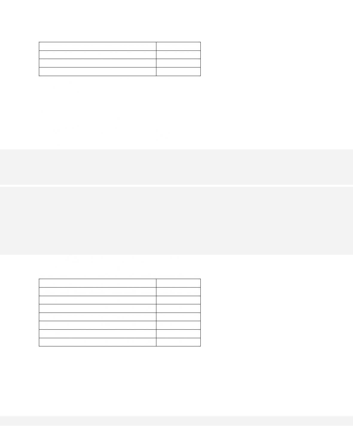
250
260
256
270
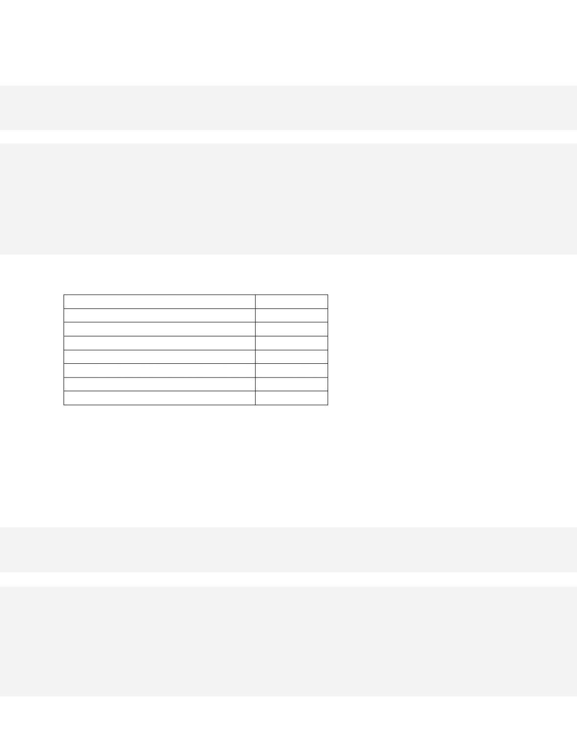
262
280
268
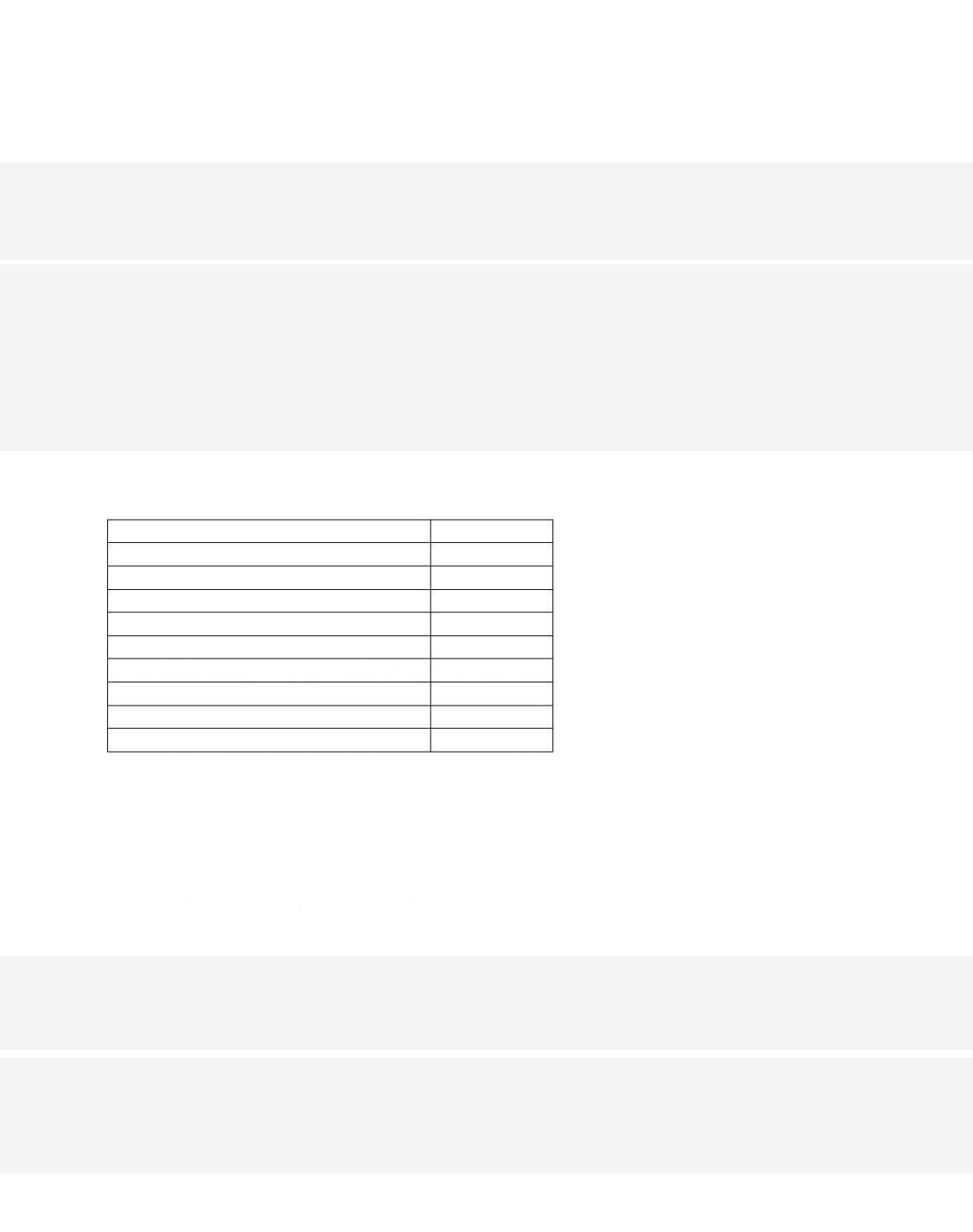
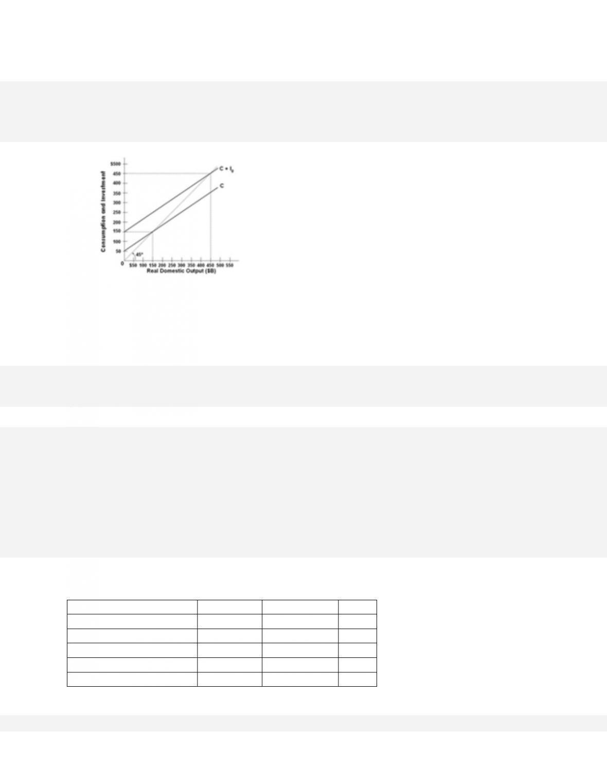
290
274
300
280
310
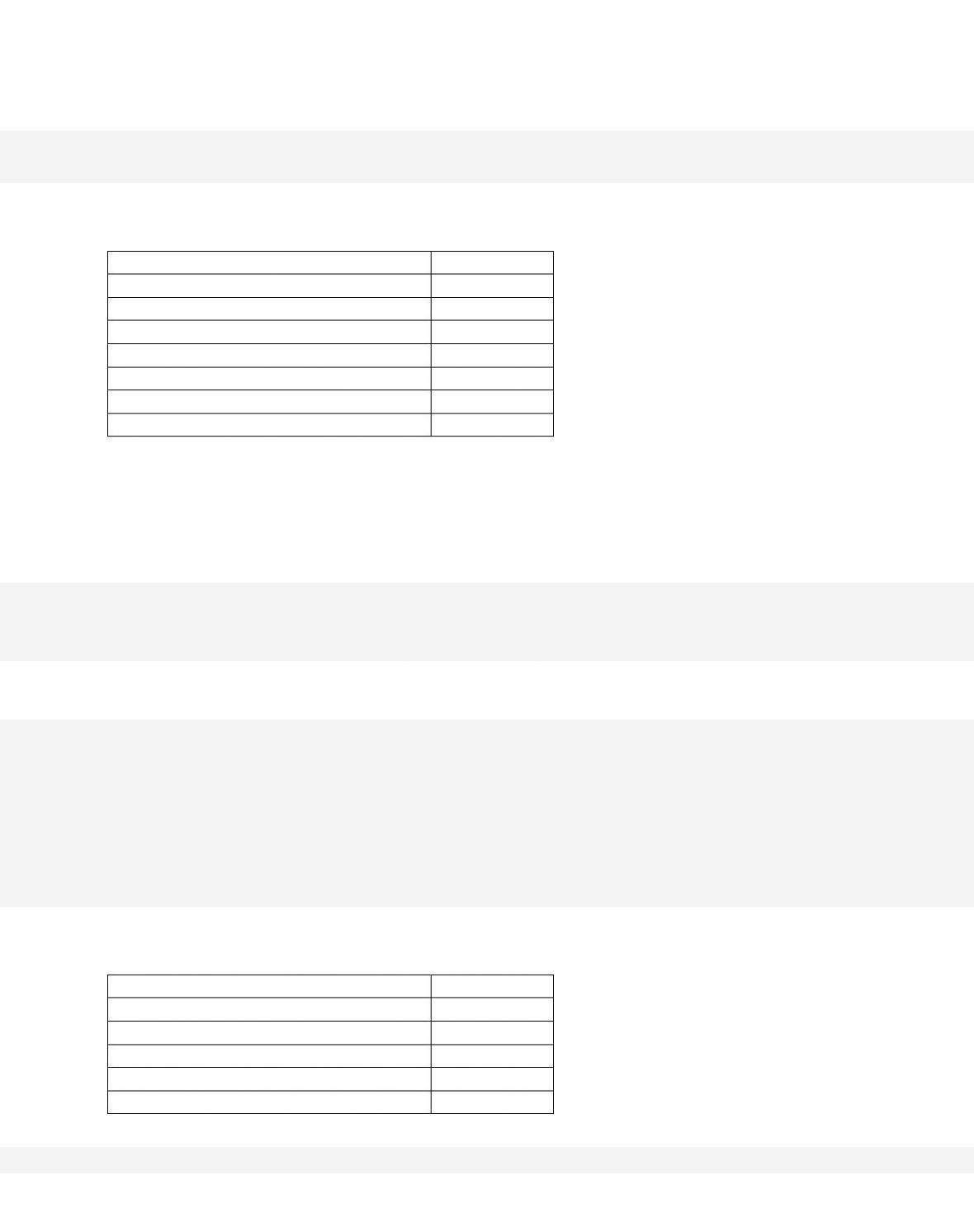
286
320
292
Refer to the table. All figures are in billions of dollars. If gross investment is $12 billion, the
equilibrium level of GDP will be
A.
$260 billion.
257.
Domestic Output or Income (GDP=DI)
Consumption
$240
$244
250
250
260
256
270
262
280
268
290
274
300
280
310
286
320
292
Refer to the table. All figures are in billions of dollars. Suppose investment is $12 billion and
the economy revises its saving plans so as to save $4 billion less at all levels of income. The
new equilibrium GDP will be
A.
$260 billion.

31-135
Copyright © 2018 McGraw-Hill Education. All rights reserved. No reproduction or distribution without the prior
written consent of McGraw-Hill Education.
Learning Objective: 31-03 Illustrate how economists combine consumption and investment to
depict an aggregate expenditures schedule for a private closed economy and how that schedule
can be used to demonstrate the economys equilibrium level of output where the total quantity of
goods produced equals the total quantity of goods purchased.
Test Bank: II
To p i c :
Equilibrium GDP: C Ig = GDP
258.
Refer to the graph for a private closed economy. In this economy, investment is
A. $50 billion.
31-136
259.
Refer to the graph for a private closed economy. The equilibrium level of GDP in this economy
is
A.
$150 billion.
260.
Refer to the graph for a private closed economy. At the equilibrium level of GDP, saving will
be
A. $50 billion.
261.
Refer to the graph for a private closed economy. At the $150-billion level of GDP,
A.
aggregate expenditures are less than real GDP, so GDP will rise.
31-138
Copyright © 2018 McGraw-Hill Education. All rights reserved. No reproduction or distribution without the prior
written consent of McGraw-Hill Education.
can be used to demonstrate the economys equilibrium level of output where the total quantity of
goods produced equals the total quantity of goods purchased.
Test Bank: II
To p i c :
Equilibrium GDP: C Ig = GDP
Type: Graph
262.
Refer to the graph for a private closed economy. When output or income is $350 billion, there
will be
A.
equilibrium GDP.
263.
Expected Rate of Return
Investment
Consumption
GDP
10%
$0
$400
$400
8
100
500
600
6
200
600
800
4
300
700
1,000
2
400
800
1,200
0
500
900
1,400
The table shows a private closed economy. All figures are in billions of dollars. If the real rate
of interest is 2 percent, then the equilibrium level of GDP will be
A.
$800 billion.
264.
Expected Rate of Return
Investment
Consumption
GDP
10%
$0
$400
$400
8
100
500
600
6
200
600
800
4
300
700
1,000
2
400
800
1,200
0
500
900
1,400
The table shows a private closed economy. All figures are in billions of dollars. An increase in
the real interest rate from 2 percent to 6 percent will
A.
decrease the equilibrium level of GDP by $200 billion.

31-140
Copyright © 2018 McGraw-Hill Education. All rights reserved. No reproduction or distribution without the prior
written consent of McGraw-Hill Education.
AACSB: Knowledge Application
Blooms: Understand
Di ff i cu l ty :
02 Medium
Learning Objective: 31-03 Illustrate how economists combine consumption and investment to
depict an aggregate expenditures schedule for a private closed economy and how that schedule
can be used to demonstrate the economys equilibrium level of output where the total quantity of
goods produced equals the total quantity of goods purchased.
Test Bank: II
To p i c :
Equilibrium GDP: C Ig = GDP
265.
Which of the following will not occur when the economy is at its equilibrium GDP level?
A.
Aggregate expenditures = GDP.
266.
In the flow of income and spending, saving and investment are, respectively,
D. income and wealth.