
30-121
Copyright © 2018 McGraw-Hill Education. All rights reserved. No reproduction or distribution without the prior
written consent of McGraw-Hill Education.
B. $450.
C. $460.
D. $470.
235.
Disposable Income
Consumption
$0
$8
80
80
160
152
240
224
320
296
400
368
The disposable income (DI) and consumption (C) schedules are for a private, closed economy.
All figures are in billions of dollars. If plotted on a graph, the slope of the consumption
schedule would be
236.

Disposable Income
Consumption
$0
$8
80
80
160
152
240
224
320
296
400
368
The disposable income (DI) and consumption (C) schedules are for a private, closed economy.
All figures are in billions of dollars. The marginal propensity to save in this economy is
237.
Disposable Income
Consumption
$0
$8
80
80
160
152
240
224
320
296
400
368
The disposable income (DI) and consumption (C) schedules are for a private, closed economy.
All figures are in billions of dollars. At the $320 billion level of disposable income, the average
propensity to save is

30-123
Copyright © 2018 McGraw-Hill Education. All rights reserved. No reproduction or distribution without the prior
written consent of McGraw-Hill Education.
B. 0.075.
C. 0.335.
D. 0.925.
238.
Disposable Income
Consumption
$0
$8
80
80
160
152
240
224
320
296
400
368
The disposable income (DI) and consumption (C) schedules are for a private, closed economy.
All figures are in billions of dollars. If consumption increases by $10 billion at each level of
disposable income, the marginal propensity to consume will
239.
The graph shows the relationship between consumption and income. Which of the following
statements is correct?
240.
The graph shows the relationship between consumption and income. The ratio LM/PL would be
a measure of the
241.
Refer to the accompanying consumption schedule. The marginal propensity to consume is
represented by
30-127
242.
Refer to the accompanying consumption schedule. The average propensity to save at income
level B is represented by
243.
Disposable Income
Consumption
$10,000
$12,000
18,000
18,000
26,000
24,000
34,000
30,000
42,000
36,000
50,000
42,000

Refer to the accompanying consumption schedule. If disposable income is $42,000, then saving
is
244.
Disposable Income
Consumption
$10,000
$12,000
18,000
18,000
26,000
24,000
34,000
30,000
42,000
36,000
50,000
42,000
Refer to the accompanying consumption schedule. The marginal propensity to consume is

30-129
Copyright © 2018 McGraw-Hill Education. All rights reserved. No reproduction or distribution without the prior
written consent of McGraw-Hill Education.
Test Bank: II
Topic:
The Income-Consumption and Income-Saving Relationships
245.
Disposable Income
Consumption
$10,000
$12,000
18,000
18,000
26,000
24,000
34,000
30,000
42,000
36,000
50,000
42,000
Refer to the accompanying consumption schedule. If disposable income were $34,000, then the
average propensity to save would be about
246. Based on OECD data for 2014, the average propensity to consume (APC) in the United
States is about

30-130
Copyright © 2018 McGraw-Hill Education. All rights reserved. No reproduction or distribution without the prior
written consent of McGraw-Hill Education.
saving.
Test Bank: II
Topic:
The Income-Consumption and Income-Saving Relationships
247. Which of the following may shift the consumption schedule upward?
248. If the consumption schedule shifts downward, and the shift was not caused by a tax
change, then the saving schedule
249. Which of the following would shift the consumption schedule downward?

30-131
Copyright © 2018 McGraw-Hill Education. All rights reserved. No reproduction or distribution without the prior
written consent of McGraw-Hill Education.
AACSB: Knowledge Application
Accessibi lity:
Keyboard Navigation
Blooms: Remember
Di f f i c u l t y :
01 Easy
Learning Objective: 30-02 List and explain factors other than income that can affect
consumption.
Test Bank: II
Topic:
Nonincome Determinants of Consumption and Saving
250. An increase in household wealth that creates a wealth effect would shift the
251. The so-called wealth effect will result in households
252. One factor that shifts the consumption schedule is household wealth. Households build
wealth by

30-132
Copyright © 2018 McGraw-Hill Education. All rights reserved. No reproduction or distribution without the prior
written consent of McGraw-Hill Education.
A. spending their current incomes.
B. spending out of their future incomes.
C. spending their incomes as they earn them.
D. not spending all their current incomes.
253. When consumers decide to increase household debt, this action will
254. Which of the following would shift the saving schedule upward?

30-133
Copyright © 2018 McGraw-Hill Education. All rights reserved. No reproduction or distribution without the prior
written consent of McGraw-Hill Education.
Topic:
Nonincome Determinants of Consumption and Saving
255. The saving schedule would be shifted upward by
256. If consumers expect prices to rise and shortages to occur in the future, then there will be a
shift
257. As the consumption and saving schedules relate to real GDP, an increase in taxes will shift

30-134
Copyright © 2018 McGraw-Hill Education. All rights reserved. No reproduction or distribution without the prior
written consent of McGraw-Hill Education.
Blooms: Remember
Di f f i c u l t y :
01 Easy
Learning Objective: 30–02 List and explain factors other than income that can affect
consumption.
Test Bank: II
Topic:
Nonincome Determinants of Consumption and Saving
258. A change in interest rates would shift the consumption schedule and the saving schedule ; a
change in taxes would shift these two schedules _.
259. A lower real interest rate typically induces consumers to
260. A change in the amount saved due to a change in income is represented by a
30-135
Copyright © 2018 McGraw-Hill Education. All rights reserved. No reproduction or distribution without the prior
written consent of McGraw-Hill Education.
C. change in the marginal propensity to save.
D. change in the marginal propensity to consume.
261.
30-136
Copyright © 2018 McGraw-Hill Education. All rights reserved. No reproduction or distribution without the prior
written consent of McGraw-Hill Education.
Test Bank: II
Topic:
Nonincome Determinants of Consumption and Saving
Type: Table
262.
263.
264. The Great Recession of 2007–2009 altered the prior behavior of consumers in the
economy by

30-138
Copyright © 2018 McGraw-Hill Education. All rights reserved. No reproduction or distribution without the prior
written consent of McGraw-Hill Education.
Blooms: Remember
Di f f i c u l t y :
01 Easy
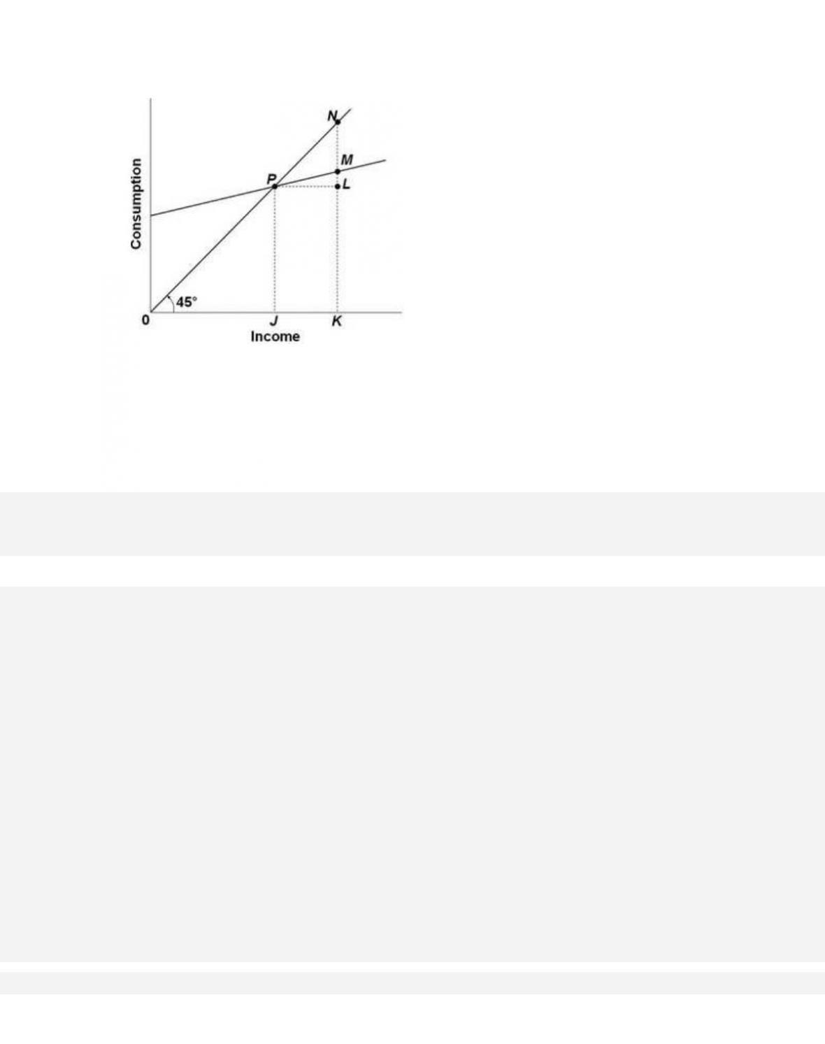
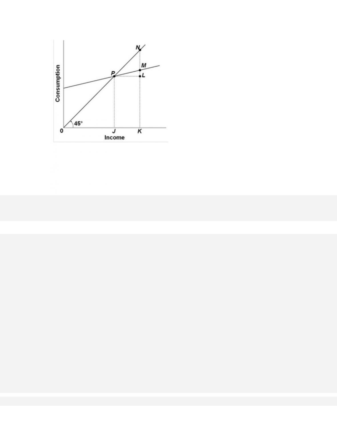
Learning Objective: 30–02 List and explain factors other than income that can affect
consumption.
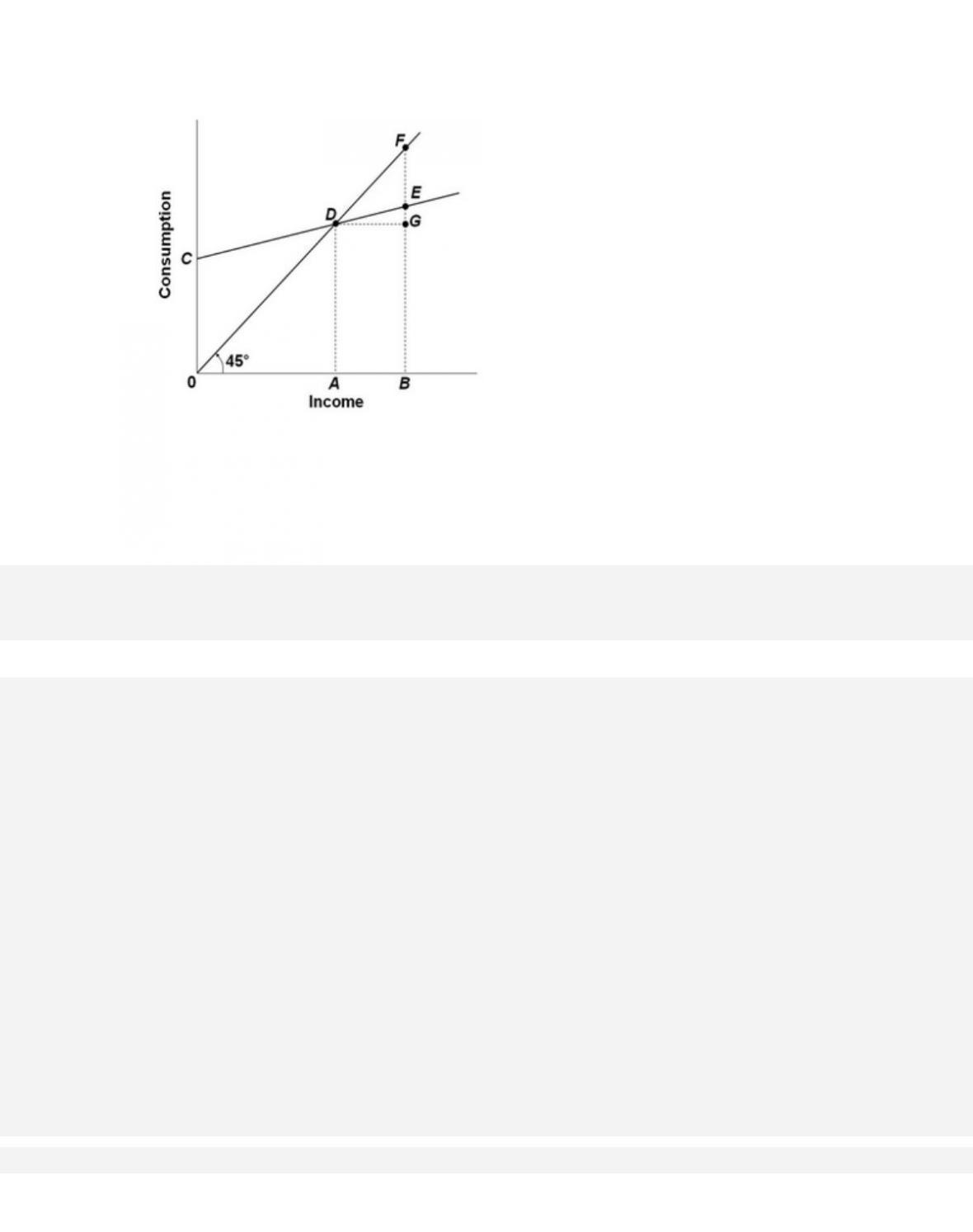
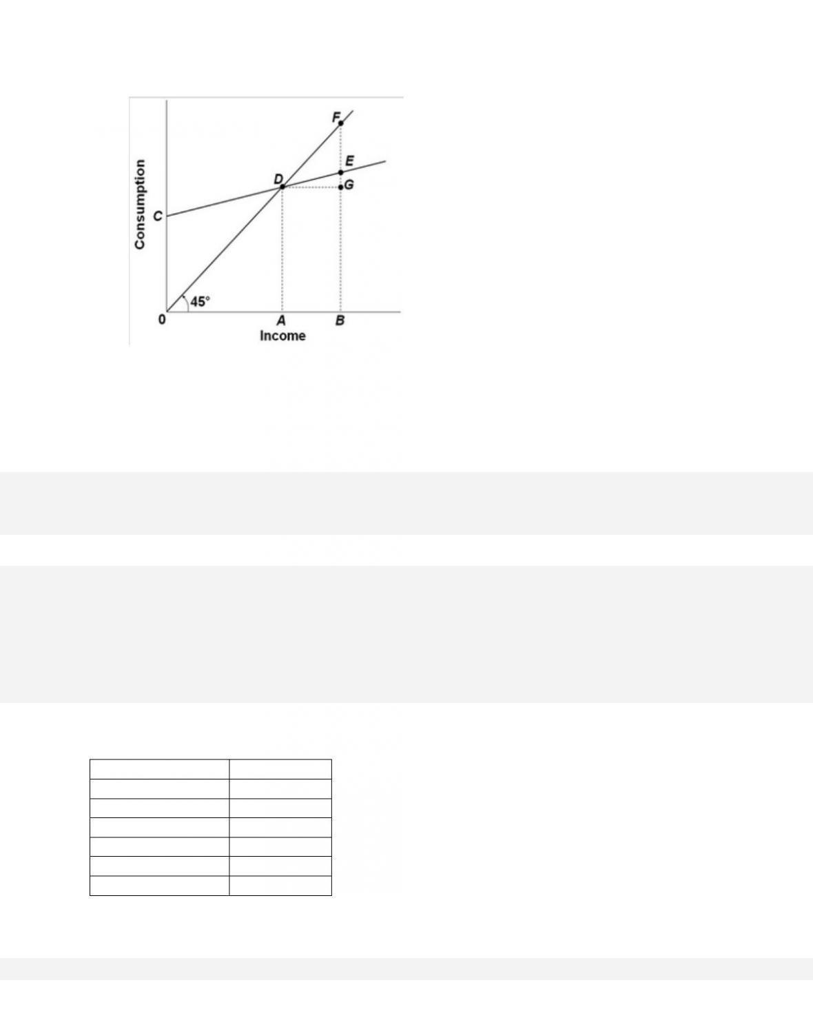
Test Bank: II
Topic:
Nonincome Determinants of Consumption and Saving
265. The so-called Paradox of Thrift that became quite obvious in the Great Recession of
2007–2009 does not refer to which of the following?
266. The Paradox of Thrift highlights the idea that
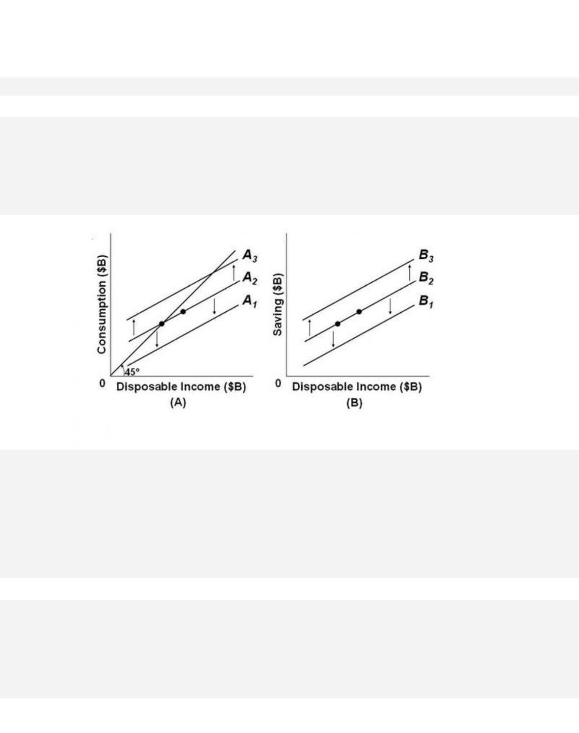
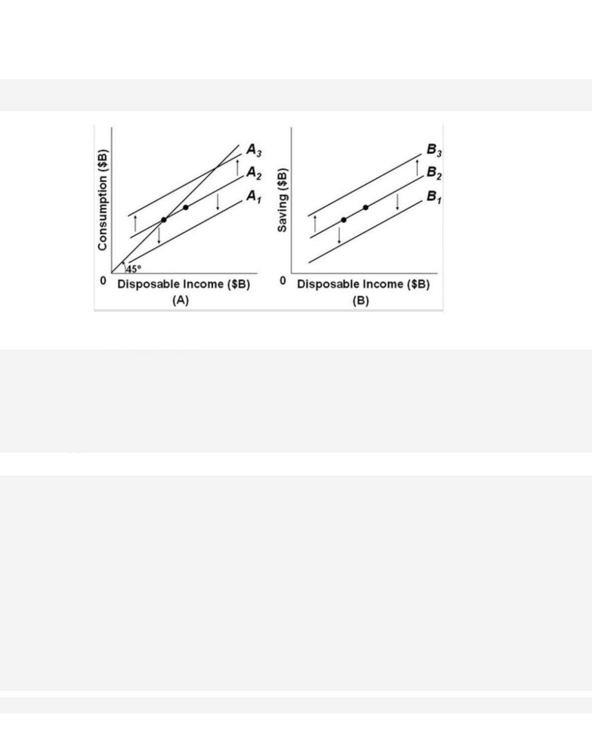
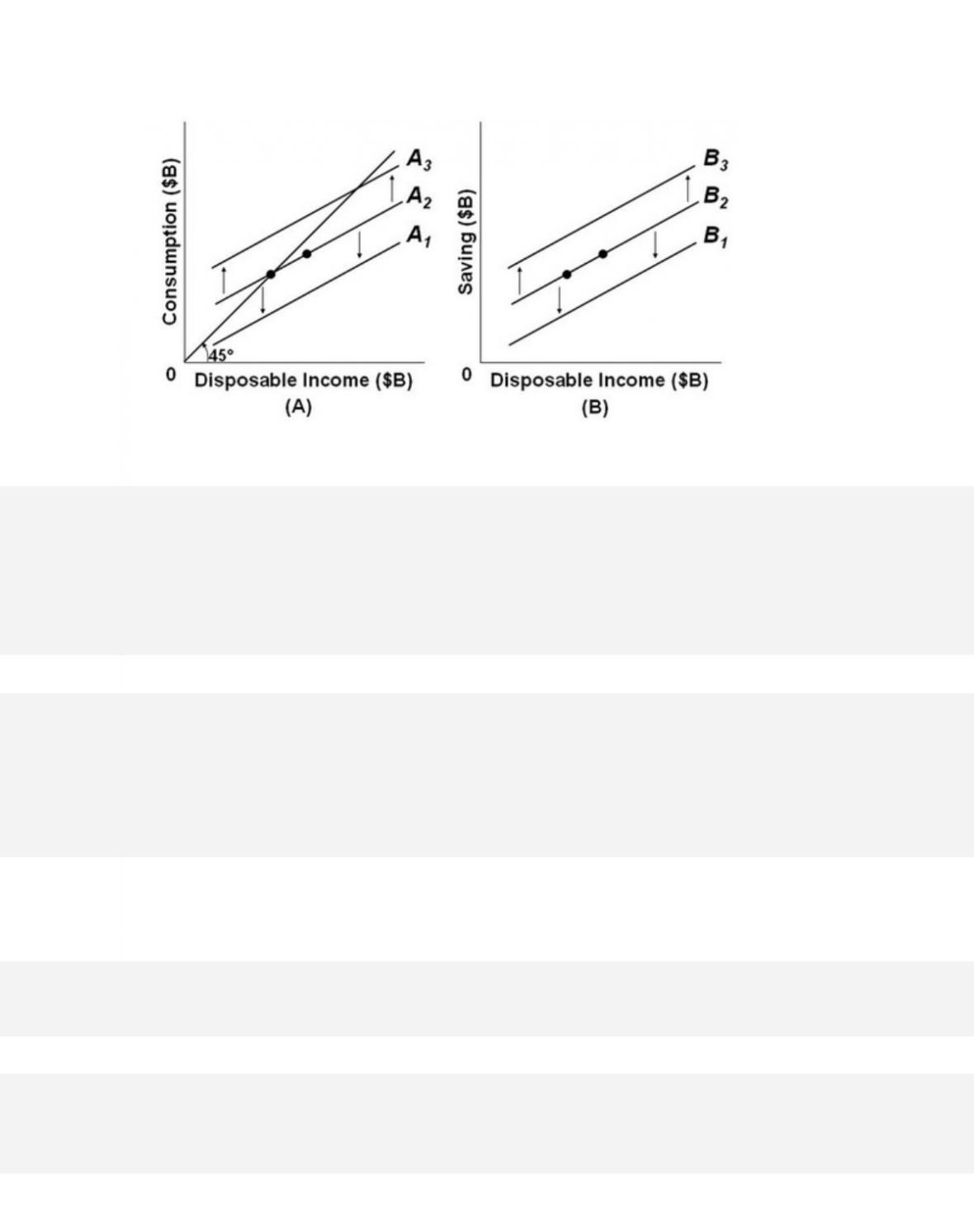
267. Two basic determinants of investment spending are

30-139
Copyright © 2018 McGraw-Hill Education. All rights reserved. No reproduction or distribution without the prior
written consent of McGraw-Hill Education.
A. consumer spending and government spending.
B. expected returns and real interest rates.
C. general price level and the level of output.
D. domestic trade and international trade.
268. An investment demand curve shows the varying amounts of investment that would be
undertaken at various levels of
269. Given the expected rate of return on all possible investment opportunities in the economy,
a(n)

30-140
Copyright © 2018 McGraw-Hill Education. All rights reserved. No reproduction or distribution without the prior
written consent of McGraw-Hill Education.
Topic:
The Interest-Rate-Investment Relationship
270. If the real interest rate increases,
271. Suppose that new computer software for accounting and analysis at a business has a useful
life of only one year and costs $200,000 before it needs to be upgraded to a new version. The
revenue generated by this software is expected to be $250,000. The expected rate of return
from this new computer software is
272. Assume there are no investment projects that will produce an expected rate of return of 8
percent or more. There are, however, $2 billion worth of investment projects with an expected
rate of return at 7 percent, and an additional $2 billion for every drop of the interest rate by 1
percent. If the real interest rate is 3 percent in this economy, the cumulative amount of
investment at the 3 percent or higher rate of return is