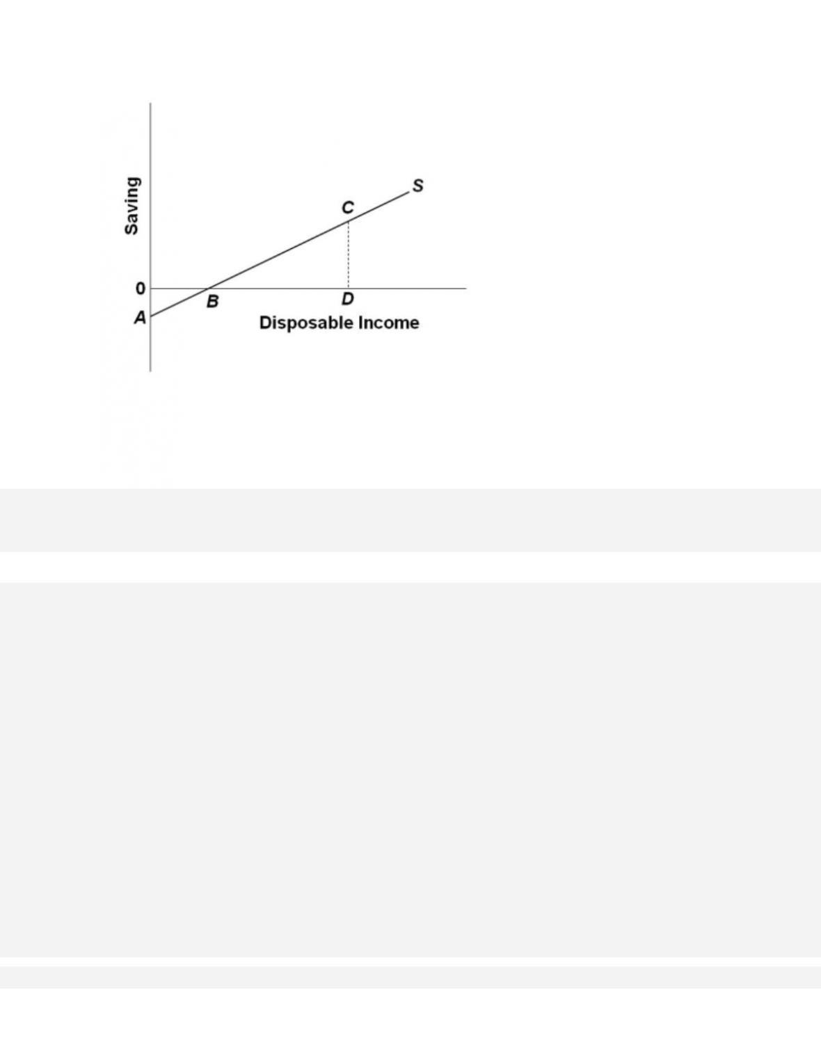
79.
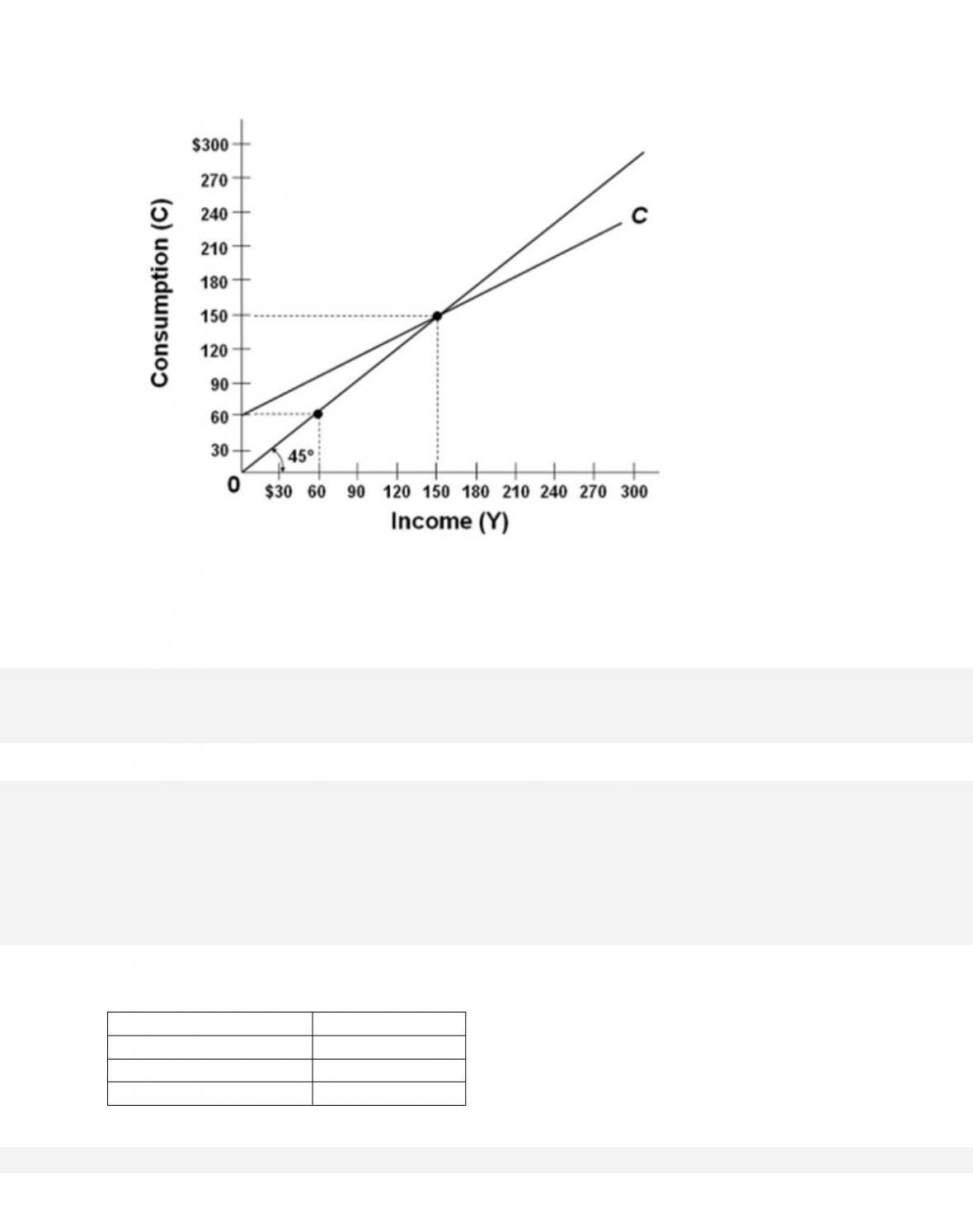
Refer to the diagram. At disposable income level D, the average propensity to save is equal to

80.
Refer to the diagram. At disposable income level D, consumption is equal to

81.
Refer to the diagram. Consumption equals disposable income when
30–44
82.
The saving schedule shown in the diagram would shift downward if, all else equal,
83.
(1)
(2)
(3)
DI
C
DI
C
DI
C
$0
$4
$0
$65
$0
$2
10
11
80
125
20
20
20
18
160
185
40
38
30
25
240
245
60
56
40
32
320
305
80
74
50
39
400
365
100
92

Refer to the given consumption schedules. DI signifies disposable income and C represents
consumption expenditures. All figures are in billions of dollars. The marginal propensity to
consume in economy (1) is
84.
(1)
(2)
(3)
DI
C
DI
C
DI
C
$0
$4
$0
$65
$0
$2
10
11
80
125
20
20
20
18
160
185
40
38
30
25
240
245
60
56
40
32
320
305
80
74
50
39
400
365
100
92
Refer to the given consumption schedules. DI signifies disposable income and C represents
consumption expenditures. All figures are in billions of dollars. The marginal propensity to
consume

30–46
Copyright © 2018 McGraw-Hill Education. All rights reserved. No reproduction or distribution without the prior
written consent of McGraw-Hill Education.
D. cannot be calculated from the data given.
85.
(1)
(2)
(3)
DI
C
DI
C
DI
C
$0
$4
$0
$65
$0
$2
10
11
80
125
20
20
20
18
160
185
40
38
30
25
240
245
60
56
40
32
320
305
80
74
50
39
400
365
100
92
Refer to the given consumption schedules. DI signifies disposable income and C represents
consumption expenditures. All figures are in billions of dollars. The marginal propensity to save
86.

30–47
(1)
(2)
(3)
DI
C
DI
C
DI
C
$0
$4
$0
$65
$0
$2
10
11
80
125
20
20
20
18
160
185
40
38
30
25
240
245
60
56
40
32
320
305
80
74
50
39
400
365
100
92
Refer to the given consumption schedules. DI signifies disposable income and C represents
consumption expenditures. All figures are in billions of dollars. At an income level of $40
billion, the average propensity to consume
87.
(1)
(2)
(3)
DI
C
DI
C
DI
C
$0
$4
$0
$65
$0
$2
10
11
80
125
20
20
20
18
160
185
40
38
30
25
240
245
60
56
40
32
320
305
80
74
50
39
400
365
100
92
Refer to the given consumption schedules. DI signifies disposable income and C represents
consumption expenditures. All figures are in billions of dollars. At an income level of $400
billion, the average propensity to save in economy (2) is
88.
(1)
(2)
(3)
DI
C
DI
C
DI
C
$0
$4
$0
$65
$0
$2
10
11
80
125
20
20
20
18
160
185
40
38
30
25
240
245
60
56
40
32
320
305
80
74
50
39
400
365
100
92
(Advanced analysis) Refer to the given consumption schedules. DI signifies disposable income
and C represents consumption expenditures. All figures are in billions of dollars. When plotted
on a graph, the vertical intercept of the consumption schedule in economy (3) is and the slope
is .

30–49
Copyright © 2018 McGraw-Hill Education. All rights reserved. No reproduction or distribution without the prior
written consent of McGraw-Hill Education.
AACSB: Knowledge Application
Blooms: Understand
D i f f i c u l t y :
02 Medium
Learning Objective: 30-01 Describe how changes in income affect consumption and
saving.
Test Bank: I
Topi c:
The Income-Consumption and Income-Saving Relationships
Type: Table
89.
(1)
(2)
(3)
DI
C
DI
C
DI
C
$0
$4
$0
$65
$0
$2
10
11
80
125
20
20
20
18
160
185
40
38
30
25
240
245
60
56
40
32
320
305
80
74
50
39
400
365
100
92
Refer to the given consumption schedules. DI signifies disposable income and C represents
consumption expenditures. All figures are in billions of dollars. Suppose that consumption
decreased by $2 billion at each level of DI in each of the three countries. We can conclude
that the
90.

(1)
(2)
(3)
DI
C
DI
C
DI
C
$0
$4
$0
$65
$0
$2
10
11
80
125
20
20
20
18
160
185
40
38
30
25
240
245
60
56
40
32
320
305
80
74
50
39
400
365
100
92
Refer to the given consumption schedules. DI signifies disposable income and C represents
consumption expenditures. All figures are in billions of dollars. A $2 billion increase in
consumption at each level of DI could be caused by
91.
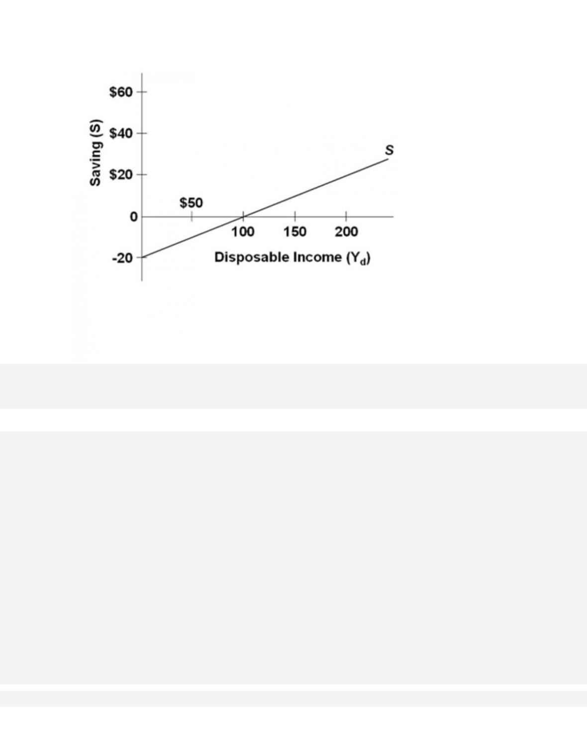
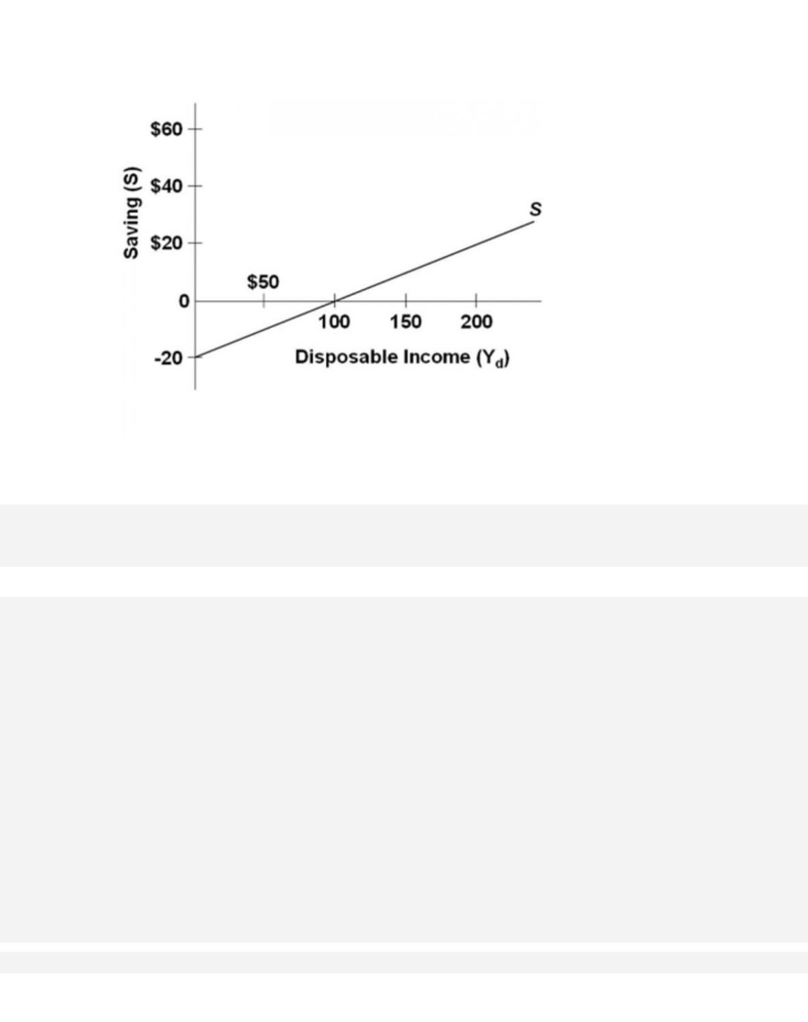
Refer to the given diagram. The marginal propensity to consume is
92.
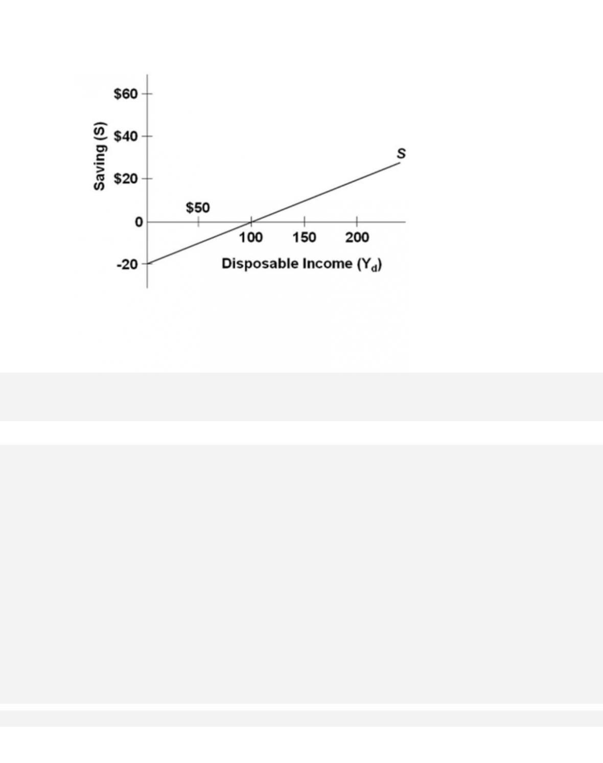
(Advanced analysis) The equation for the given saving schedule is
93.
Refer to the diagram. The average propensity to consume
30–54
94.
Refer to the diagram. The break-even level of income is
95.
Refer to the diagram. The marginal propensity to consume is
30–56
96.
(Advanced analysis) Refer to the diagram. The equation for the consumption schedule is
97.
Disposable Income (Yd)
Consumption (C)
$0
$40
100
100
200
160

300
220
400
280
(Advanced analysis) Which of the following equations correctly represents the given data?
98.
Disposable Income (Yd)
Consumption (C)
$0
$40
100
100
200
160
300
220
400
280
(Advanced analysis) Which of the following equations represents the saving schedule implicit
in the given data?

30–58
Copyright © 2018 McGraw-Hill Education. All rights reserved. No reproduction or distribution without the prior
written consent of McGraw-Hill Education.
Blooms: Understand
D i f f i c u l t y :
02 Medium
Learning Objective: 30-01 Describe how changes in income affect consumption and
saving.
Test Bank: I
Topi c:
The Income-Consumption and Income-Saving Relationships
Type: Table
99. The investment demand curve portrays an inverse (negative) relationship between
100. The investment demand slopes downward and to the right because lower real interest rates
101. Other things equal, a decrease in the real interest rate will

30–59
Copyright © 2018 McGraw-Hill Education. All rights reserved. No reproduction or distribution without the prior
written consent of McGraw-Hill Education.
D. move the economy downward along its existing investment demand curve.
102. Suppose that a new machine tool having a useful life of only one year costs $80,000.
Suppose, also, that the net additional revenue resulting from buying this tool is expected to be
$96,000. The expected rate of return on this tool is
103. Assume a machine that has a useful life of only one year costs $2,000. Assume, also, that
net of such operating costs as power, taxes, and so forth, the additional revenue from the output
of this machine is expected to be $2,300. The expected rate of return on this machine is

104. Assume a machine that has a useful life of only one year costs $2,000. Assume, also, that
net of such operating costs as power, taxes, and so forth, the additional revenue from the output
of this machine is expected to be $2,300. If the firm finds it can borrow funds at an interest rate
of 10 percent, the firm should
105. The relationship between the real interest rate and investment is shown by the
106. Given the expected rate of return on all possible investment opportunities in the economy,