
20–41
Copyright © 2018 McGraw-Hill Education. All rights reserved. No reproduction or distribution without the prior
written consent of McGraw-Hill Education.
Learning Objective: 20–08 Discuss the probable incidence of U.S. taxes and how the
distribution of income between rich and poor is affected by government taxes, transfers, and
spending.
Test Bank: I
Topi c :
Probable Incidence of U.S. Taxes
82. The U.S. tax-transfer system (as distinct from the tax system alone) is
D. regressive.
83. In 2011, the 20 percent of families with the lowest incomes paid an effective average
federal tax rate (on all federal taxes) of about , whereas the 20 percent of families with the
highest incomes paid an effective average tax rate of about .
A. 5.5 percent; 50 percent
20–42
84. According to the Organization for Economic Cooperation and Development (OECD),
D. the U.S. tax system has the same degree of progressivity as those of many developing
nations.
85. The incidence of a tax pertains to
A. the degree to which it alters the distribution of income.
86.
Quantity Demanded
Price
Quantity Supplied
1,500
$10
3,500
2,000
9
3,000
2,500
8
2,500
3,000
7
2,000
3,500
6
1,500
The table gives demand and supply data for a competitive market. If government levies a per–
unit excise tax of $1 on suppliers of this product, equilibrium price and quantity will be
A. $9 and 3,000.
87.
Quantity Demanded
Price
Quantity Supplied
1,500
$10
3,500
2,000
9
3,000
2,500
8
2,500
3,000
7
2,000
3,500
6
1,500
The table gives demand and supply data for a competitive market. If government provides a
per-unit subsidy of $2 to suppliers of this product, equilibrium price and quantity will be

20–44
Copyright © 2018 McGraw-Hill Education. All rights reserved. No reproduction or distribution without the prior
written consent of McGraw-Hill Education.
efficiency losses caused by taxes.
Test Bank: I
Topi c :
Tax Incidence and Efficiency Loss
Type: Table
88. Assume the Environmental Protection Agency imposes an excise tax on polluting firms. In
which of the following situations would we expect the additional costs to be borne most heavily
by consumers?
A. Demand is highly elastic and supply is highly inelastic.
89. If the demand for a product is perfectly elastic and supply is upsloping, a $1 excise tax per
unit on suppliers will
D. raise price by $1.
90. If the supply of a product is perfectly elastic and demand is downsloping, an excise tax of
$2 per unit will increase price by
A. more than $2.

20–45
Copyright © 2018 McGraw-Hill Education. All rights reserved. No reproduction or distribution without the prior
written consent of McGraw-Hill Education.
B. less than $2.
C. $2 and increase equilibrium output.
D. $2 and reduce equilibrium output.
91. Suppose that government imposes a specific excise tax on product X of $2 per unit and that
the price elasticity of demand for X is unitary (coefficient = 1). If the incidence of the tax is
such that the producers of X pay $1.75 of the tax and the consumers pay $.25, we can
conclude that the
D. demand for X is highly elastic.
92. Suppose that government imposes a specific excise tax on product X of $2 per unit and that
the price elasticity of demand for X is unitary (coefficient = 1). If the incidence of the tax is
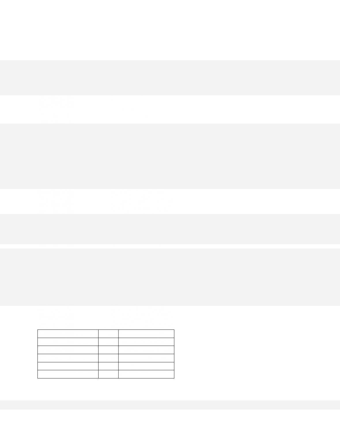
such that consumers pay $1.80 of the tax and the producers pay $.20, we can conclude that the
A. supply of X is highly inelastic.

20–46
Copyright © 2018 McGraw-Hill Education. All rights reserved. No reproduction or distribution without the prior
written consent of McGraw-Hill Education.
Difficulty:
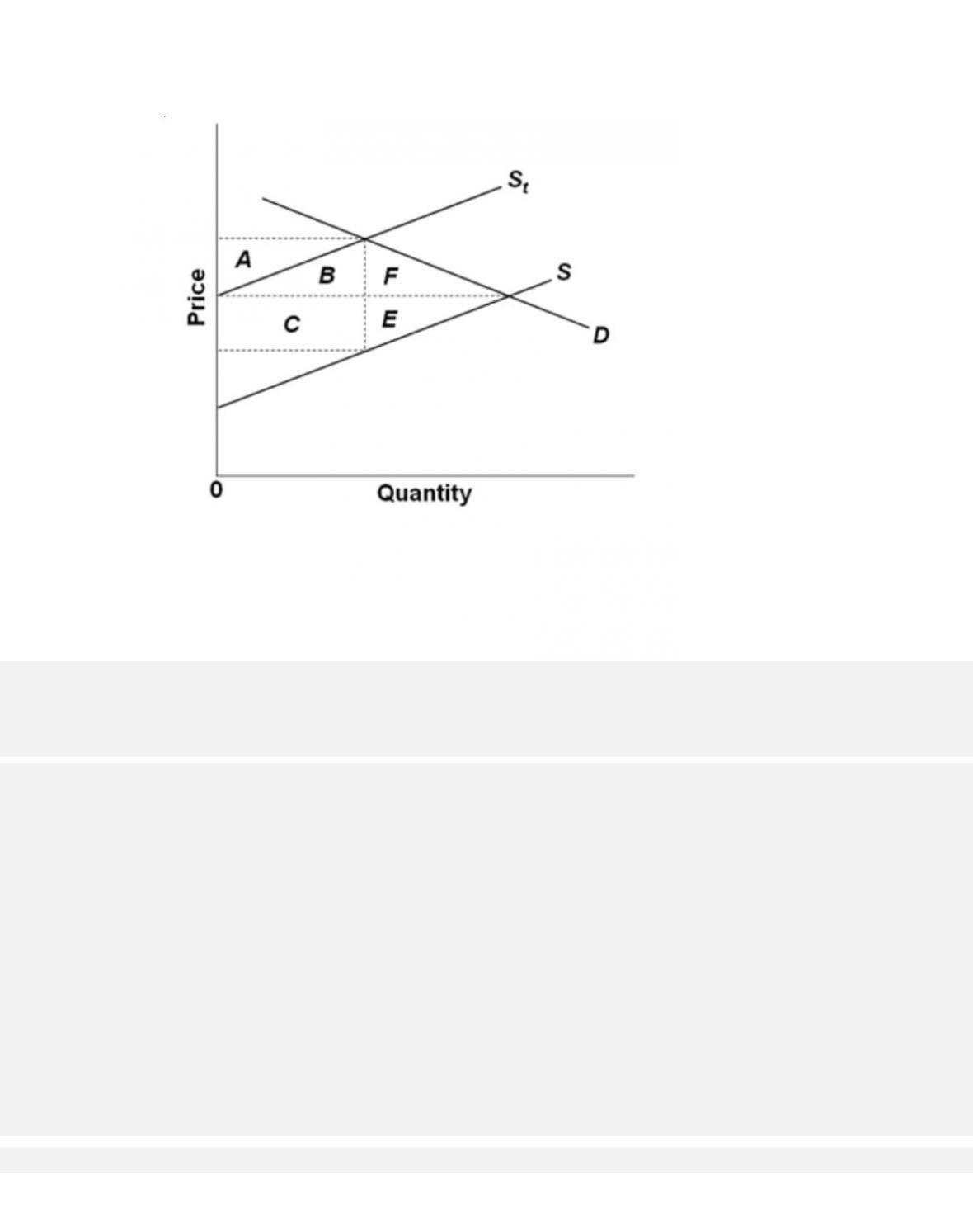
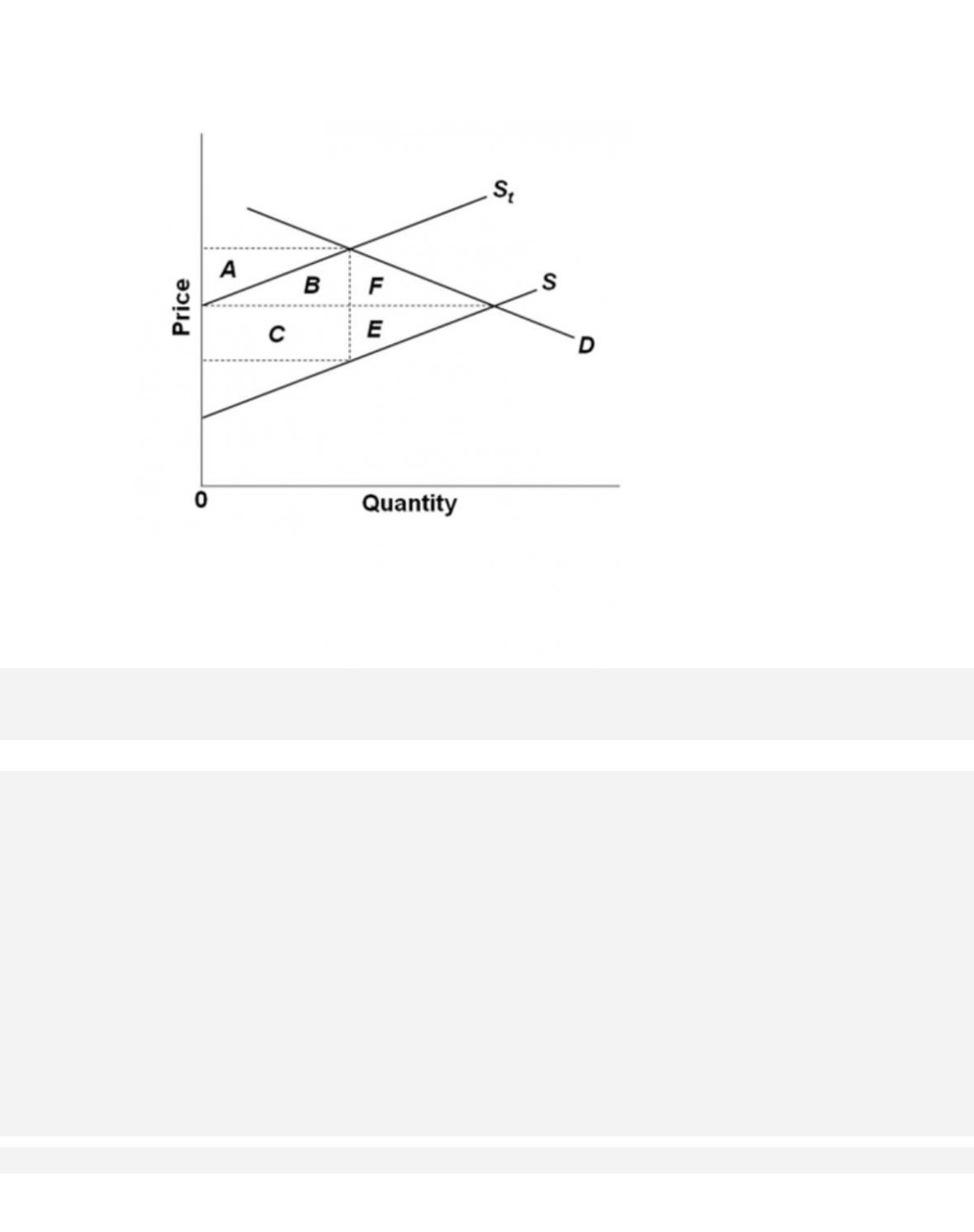
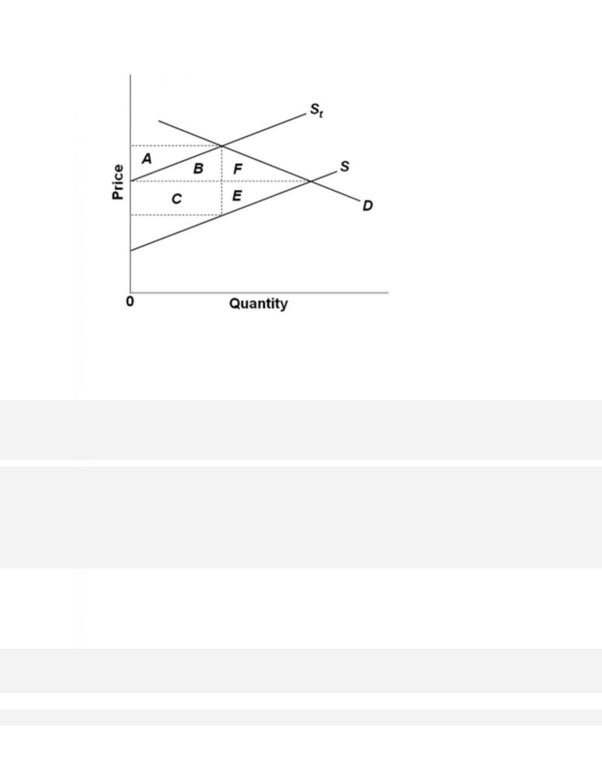
02 Medium
Learning Objective: 20–07 Explain the principles relating to tax shifting, tax incidence, and the
efficiency losses caused by taxes.
Test Bank: I
Topi c :
Tax Incidence and Efficiency Loss
93. Suppose that government imposes a specific excise tax on product X of $2 per unit and that
the price elasticity of supply of X is unitary (coefficient = 1). If the incidence of the tax is such
that the producers of X pay $1.90 of the tax and the consumers pay $.10, we can conclude that
the
A. supply of X is highly inelastic.
94. Suppose that government imposes a specific excise tax on product X of $2 per unit and that
the price elasticity of supply of X is unitary (coefficient = 1). If the incidence of the tax is such
that the consumers of X pay $1.85 of the tax and the producers pay $0.15, we can conclude
that the
A. supply of X is highly inelastic.
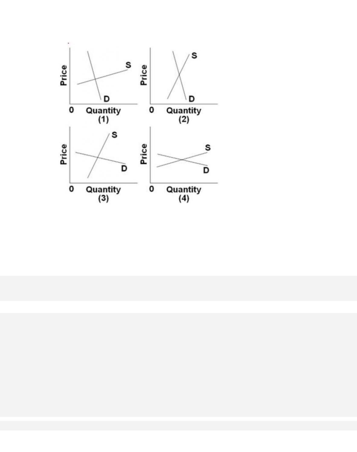
95.
In which of the given market situations will the largest portion of an excise tax of a specified
amount per unit of output be borne by producers?
A. 4
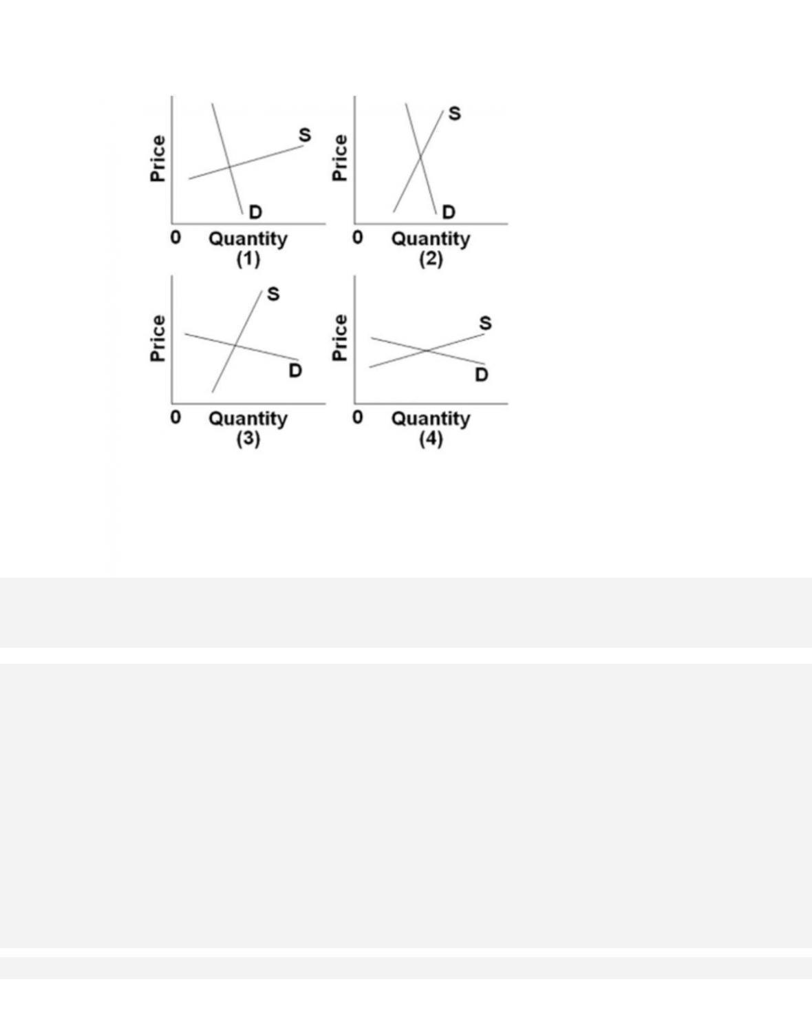
96.
In which of the given market situations will the largest portion of an excise tax of a specified
amount per unit of output be borne by buyers?
A. 4
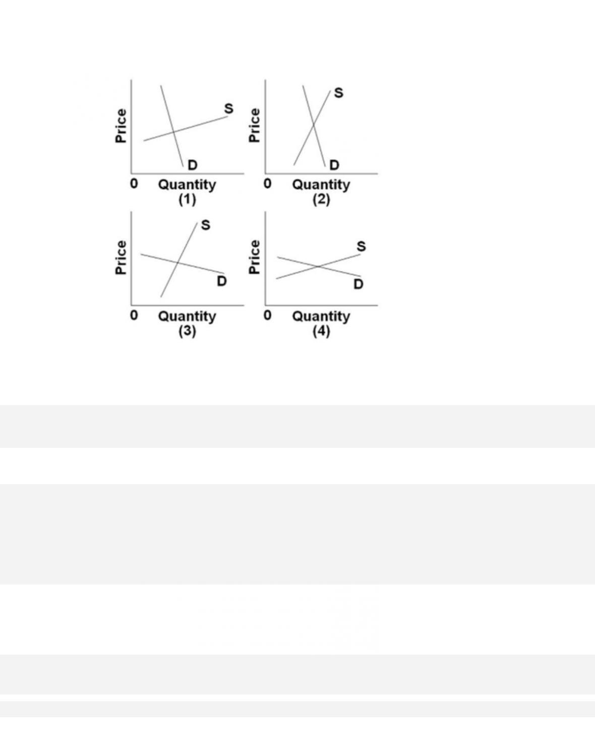
97.
In which of the given market situations will the efficiency loss of an excise tax be the greatest?
D. 2
98. Assume the demand for automobile tires is highly inelastic and that the supply is highly
elastic. The burden of a $2 excise tax on each tire will be
A. borne by resource suppliers that provide the inputs for manufacturing tires.

20–50
Copyright © 2018 McGraw-Hill Education. All rights reserved. No reproduction or distribution without the prior
written consent of McGraw-Hill Education.
D. borne primarily by sellers of tires.
99. Assume the supply curve for product X is perfectly elastic and that government imposes a
$2-per-unit excise tax. We can conclude that the resulting
A. increase in output will be greater the less elastic the demand curve.
100. If the demand for a product is perfectly inelastic and the supply curve is upsloping, a $1
excise tax per unit of output will
A. raise the price by less than $1.
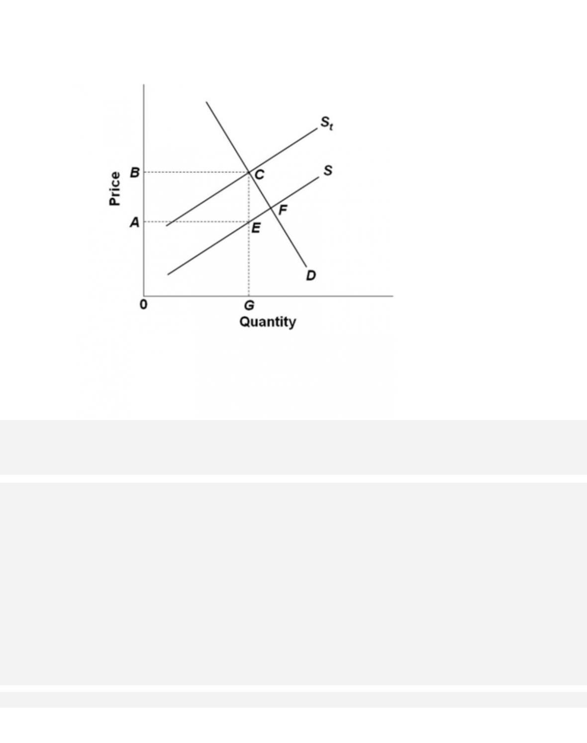
101.
In the figure, S is the before-tax supply curve and St is the supply curve after an excise tax is
imposed. The total tax collection from this excise tax will be area
A. ABCE + ECF.
102.
In the figure, S is the before-tax supply curve and St is the supply curve after an excise tax is
imposed. The efficiency loss of this tax will be area
A. ABCE.
20–53
103.
In the figure, S is the before-tax supply curve and St is the supply curve after an excise tax is
imposed. The burden of this tax is borne
A. equally by consumers and producers.
104. The more inelastic are demand and supply, the
A. larger is the efficiency loss of an excise tax.

20–54
105. If the demand for a product is perfectly inelastic, the incidence of an excise tax will be
D. mostly on the seller.
106. The efficiency loss of a tax is the idea that
A. in addition to taking income from the citizenry, taxes also increase the rate of inflation.
107. The greater the elasticity of supply of and demand for a good, the

A. smaller will be the efficiency loss of an excise tax on the good.
108. The efficiency loss of a tax is
D. the total tax revenue minus the output loss caused by the tax.
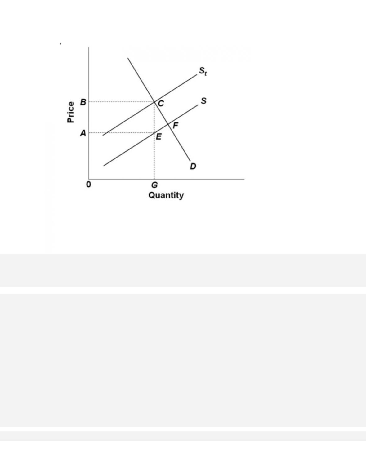
109.
In the diagram, S is the before-tax supply curve and St is the supply curve after an excise tax is
imposed. The total tax payment to government is shown by area(s)
A. A only.

110.
In the diagram, S is the before-tax supply curve and St is the supply curve after an excise tax is
imposed. The total amount of the tax paid by consumers is shown by areas
A. A + B + F.
111.
In the diagram, S is the before-tax supply curve and St is the supply curve after an excise tax is
imposed. The total amount of the tax paid by producers is shown by area(s)
A. A + B + F.
20–59
112.
In the diagram, S is the before-tax supply curve and St is the supply curve after an excise tax is
imposed. The efficiency loss of the tax is shown by areas
113. (Advanced analysis) The equations for the demand and supply curves for a particular
product are P = 10 − 0.4Q and P = 2 + 0.4Q, where P is price and Q is quantity expressed in
units of 100. After an excise tax is imposed on the product, the supply equation is P = 3 +
0.4Q. The excise tax on each unit of the product

20–60
Copyright © 2018 McGraw-Hill Education. All rights reserved. No reproduction or distribution without the prior
written consent of McGraw-Hill Education.
C. is $3.
D. cannot be determined with the information given.
114. (Advanced analysis) The equations for the demand and supply curves for a particular
product are P = 10 − 0.4Q and P = 2 + 0.4Q, where P is price and Q is quantity expressed in
units of 100. After an excise tax is imposed on the product, the supply equation is P = 3 +
0.4Q.The equilibrium quantity before the excise tax is imposed is
A. 800 units.
115. (Advanced analysis) The equations for the demand and supply curves for a particular
product are P = 10 − 0.4Q and P = 2 + 0.4Q, where P is price and Q is quantity expressed in
units of 100. After an excise tax is imposed on the product, the supply equation is P = 3 +
0.4Q. The equilibrium quantity after the excise tax is imposed is
A. 750 units.