42.
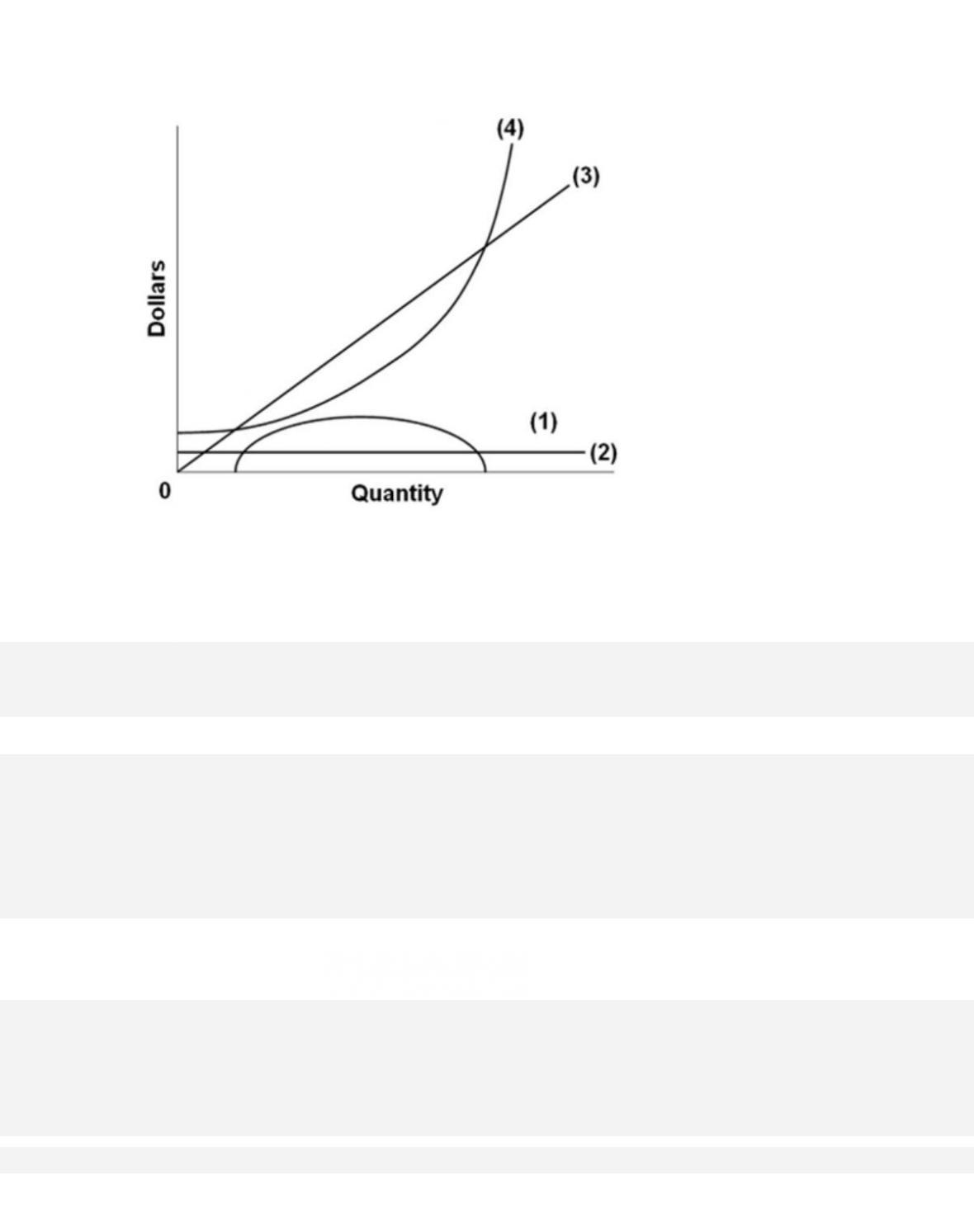
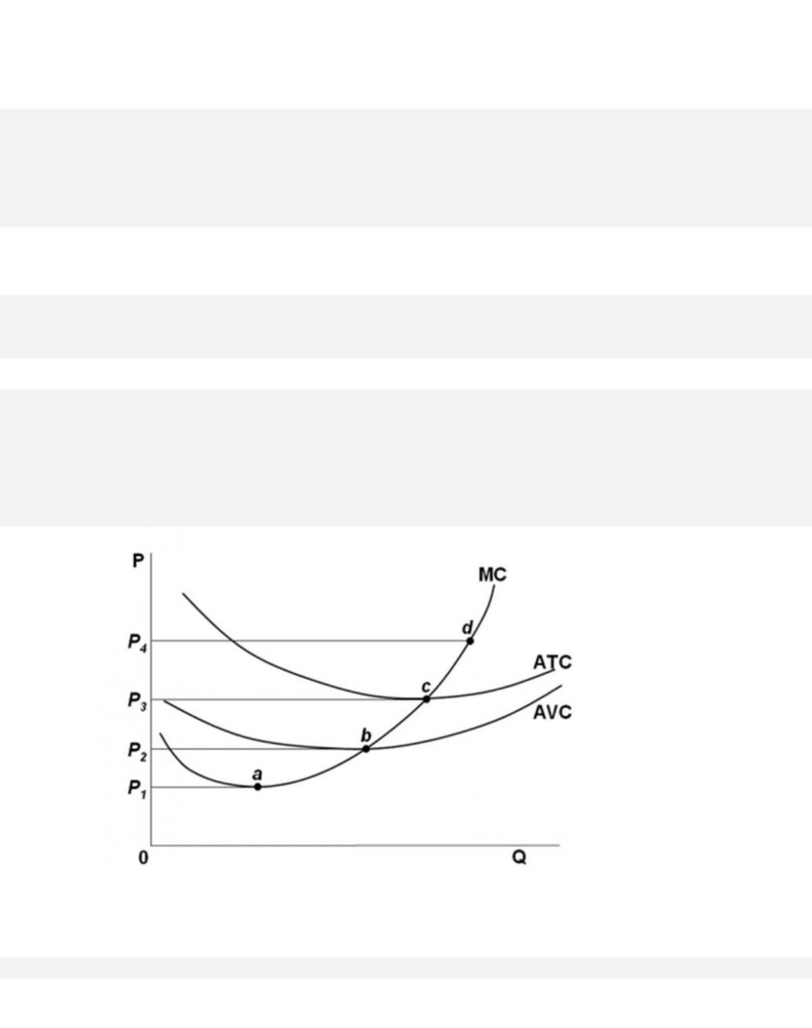
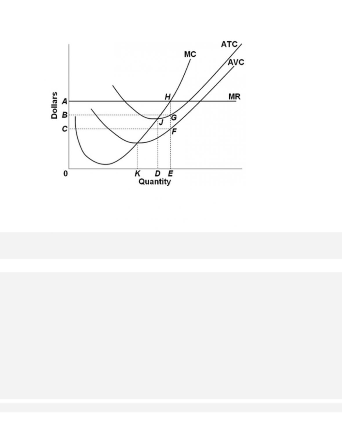
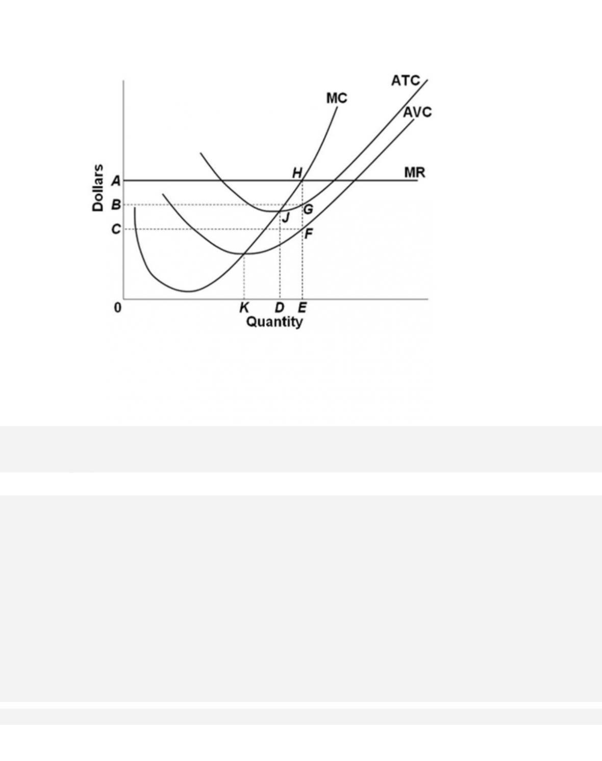
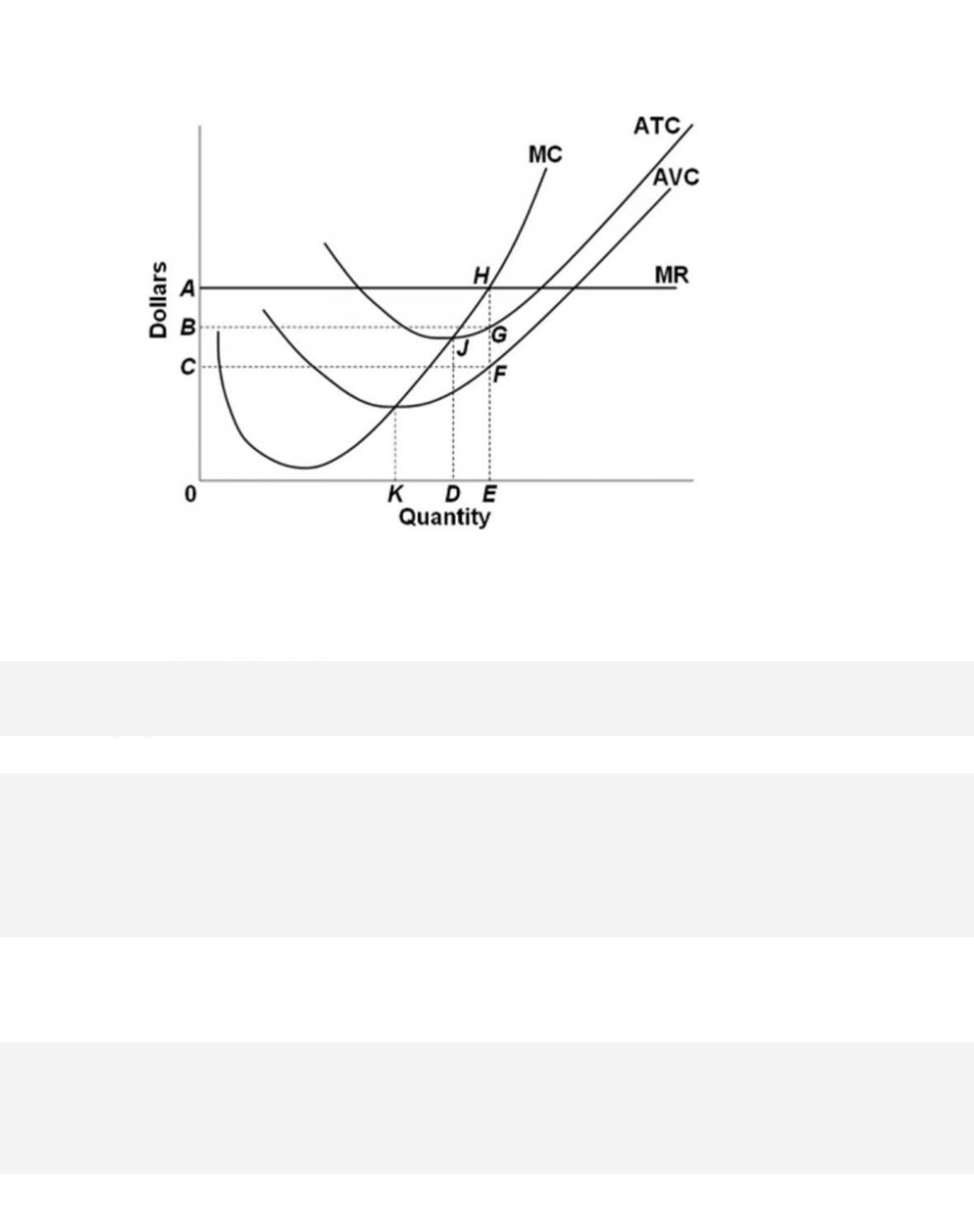
The firm represented by the diagram would maximize its profit where
43.
A firm reaches a break-even point (normal profit position) where

10–22
Copyright © 2018 McGraw-Hill Education. All rights reserved. No reproduction or distribution without the prior
written consent of McGraw-Hill Education.
AACSB: Knowledge Application
A c c e s s i b i l i t y :
Keyboard Navigation
Blooms: Understand
D i f f i c u lt y :
02 Medium
Learning Objective: 10–04 Convey how purely competitive firms can use the total-revenue–
total-cost approach to maximize profits or minimize losses in the short run.
Test Bank: I
T o p i c :
Profit Maximization in the Short Run: Total-Revenue–Total-Cost Approach
44.
The MR = MC rule applies
45.
When a firm is maximizing profit, it will necessarily be
46.
The MR = MC rule can be restated for a purely competitive seller as P = MC because

10–23
Copyright © 2018 McGraw-Hill Education. All rights reserved. No reproduction or distribution without the prior
written consent of McGraw-Hill Education.
B.
the firm’s average revenue curve is downsloping.
C.
the market demand curve is downsloping.
D.
the firm‘s marginal revenue and total revenue curves will coincide.
47.
In the short run, the individual competitive firm’s supply curve is that segment of the
48.
Which of the following is not a valid generalization concerning the relationship between
price and costs for a purely competitive seller in the short
run?

10–24
Copyright © 2018 McGraw-Hill Education. All rights reserved. No reproduction or distribution without the prior
written consent of McGraw-Hill Education.
its supply curve.
Test Bank: I
T o p i c :
Marginal Cost and Short-Run Supply
49.
Assume the XYZ Corporation is producing 20 units of output. It is selling this output in a
purely competitive market at $10 per unit. Its total fixed
costs are $100 and its average
variable cost is $3 at 20 units of output. This corporation
50.
A purely competitive firm’s short-run supply curve is
51.
Suppose you find that the price of your product is less than minimum AVC. You should

10–25
Copyright © 2018 McGraw-Hill Education. All rights reserved. No reproduction or distribution without the prior
written consent of McGraw-Hill Education.
C. close down because, by producing, your losses will exceed your total fixed costs.
D. close down because total revenue exceeds total variable cost.
52.
If a purely competitive firm shuts down in the short run,
53.
A purely competitive firm should produce in the short run if its total revenue is sufficient to
cover its
10–26
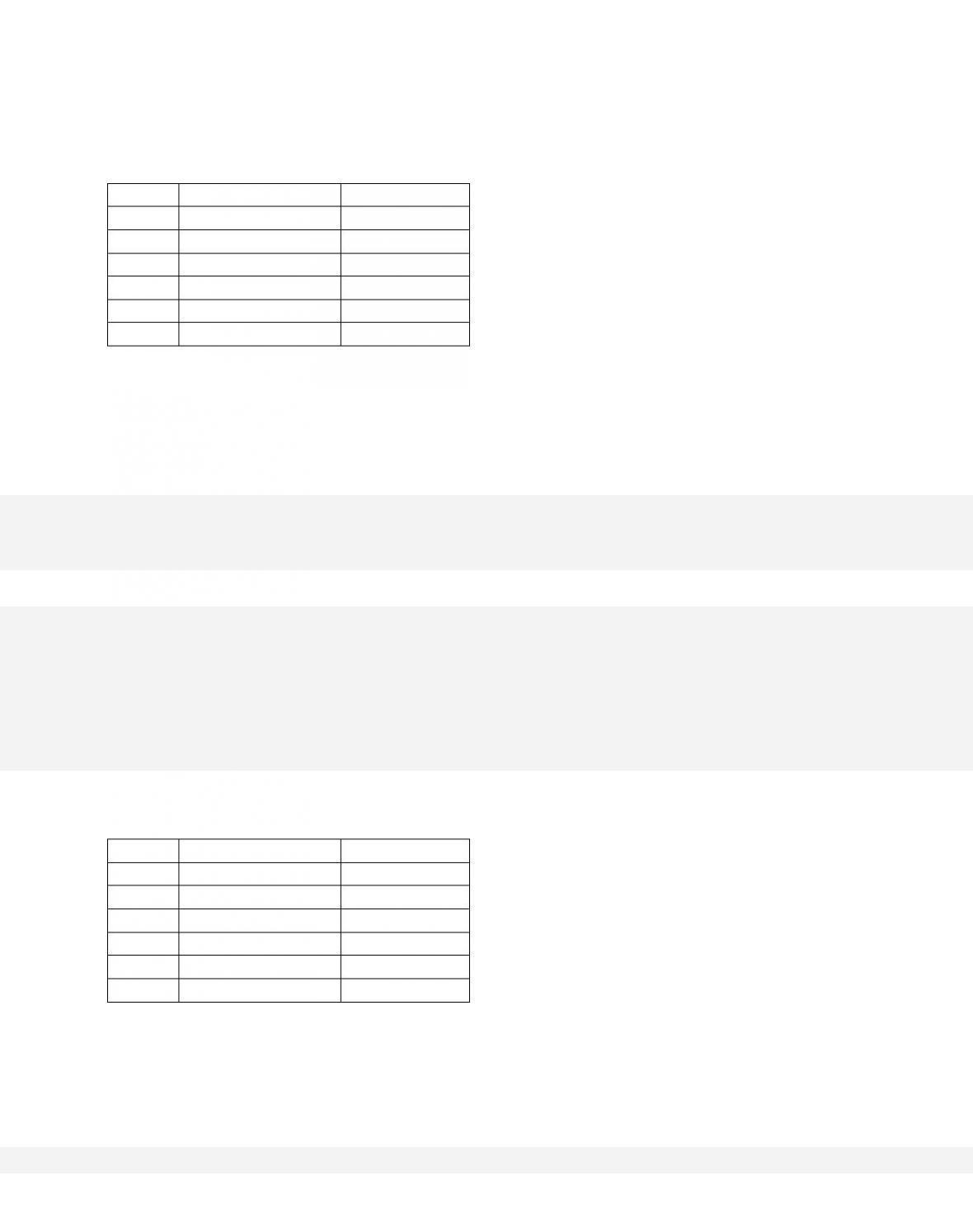
54.
Output
Marginal Revenue
Marginal Cost
0
—
—
1
$16
$10
2
16
9
3
16
13
4
16
17
5
16
21
The data in the accompanying table indicates that this firm is selling its output in a(n)
55.
Output
Marginal Revenue
Marginal Cost
0
—
—
1
$16
$10
2
16
9
3
16
13
4
16
17
5
16
21
Refer to the data in the accompanying table. If the firm’s minimum average variable cost is $10,
the firm’s profit-maximizing level of output would be
10–27
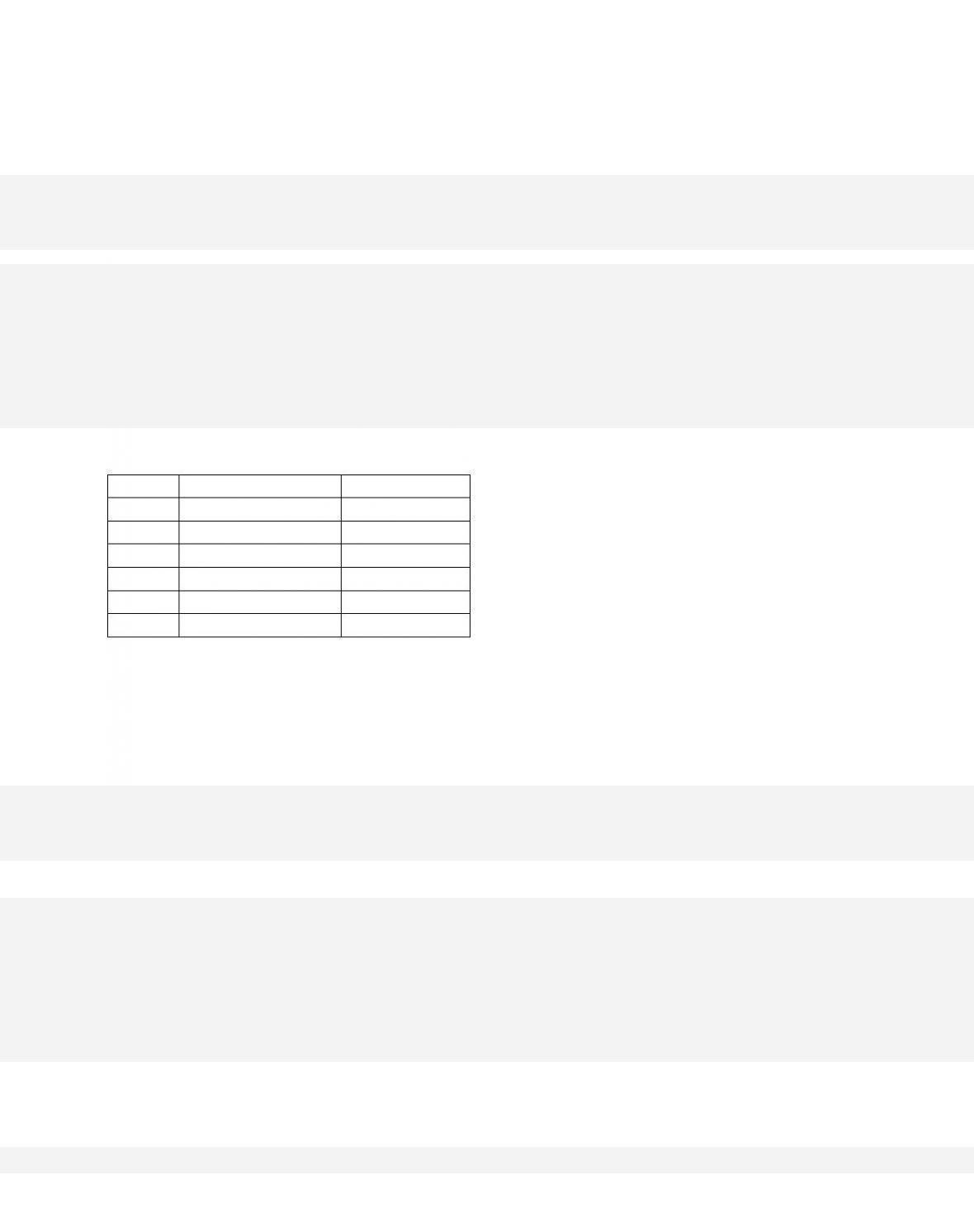
56.
Output
Marginal Revenue
Marginal Cost
0
—
—
1
$16
$10
2
16
9
3
16
13
4
16
17
5
16
21
Refer to the data in the accompanying table. At the profit-maximizing output, the firm’s total
revenue is
57.
Output
Marginal Revenue
Marginal Cost
0
—
—
1
$16
$10
2
16
9
3
16
13
4
16
17
5
16
21
Refer to the data in the accompanying table. Assuming total fixed costs equal to zero, the firm’s
58.
In the short run, a purely competitive firm will always make an economic profit if

59.
Suppose that at 500 units of output, marginal revenue is equal to marginal cost. The firm is
selling its output at $5 per unit, and average total cost at
500 units of output is $6. On the basis
of this information, we
60.
If a firm is confronted with economic losses in the short run, it will decide whether or not
to produce by comparing
61.
A firm finds that at its MR = MC output, its TC = $1,000, TVC = $800, TFC = $200, and
total revenue is $900. This firm should
10–30
Copyright © 2018 McGraw-Hill Education. All rights reserved. No reproduction or distribution without the prior
written consent of McGraw-Hill Education.
A c c e s s i b i l i t y :
Keyboard Navigation
Blooms: Understand
D i f f i c u lt y :
02 Medium
Learning Objective: 10–05 Explain how purely competitive firms can use the marginal-revenue–
marginal-cost approach to maximize profits or minimize losses in the short run.
Test Bank: I
T o p i c :
Profit Maximization in the Short Run: Marginal-Revenue–Marginal-Cost Approach
62.
The lowest point on a purely competitive firm’s short-run supply curve corresponds to
63.
Refer to the diagram for a purely competitive producer. The lowest price at which the firm
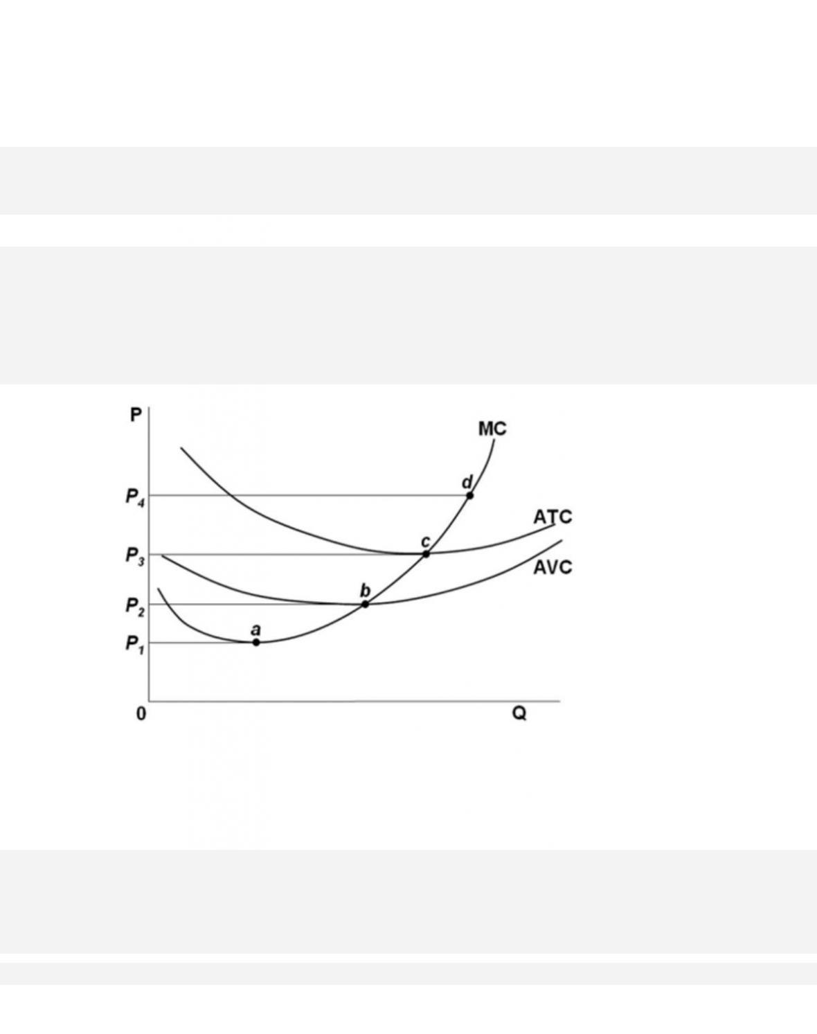
should produce (as opposed to shutting down) is
64.
Refer to the diagram for a purely competitive producer. The firm will produce at a loss at all
prices
65.
Refer to the diagram for a purely competitive producer. If product price is P3,
10–33
Copyright © 2018 McGraw-Hill Education. All rights reserved. No reproduction or distribution without the prior
written consent of McGraw-Hill Education.
T o p i c :
Profit Maximization in the Short Run: Marginal-Revenue–Marginal-Cost Approach
Type: Graph
66.
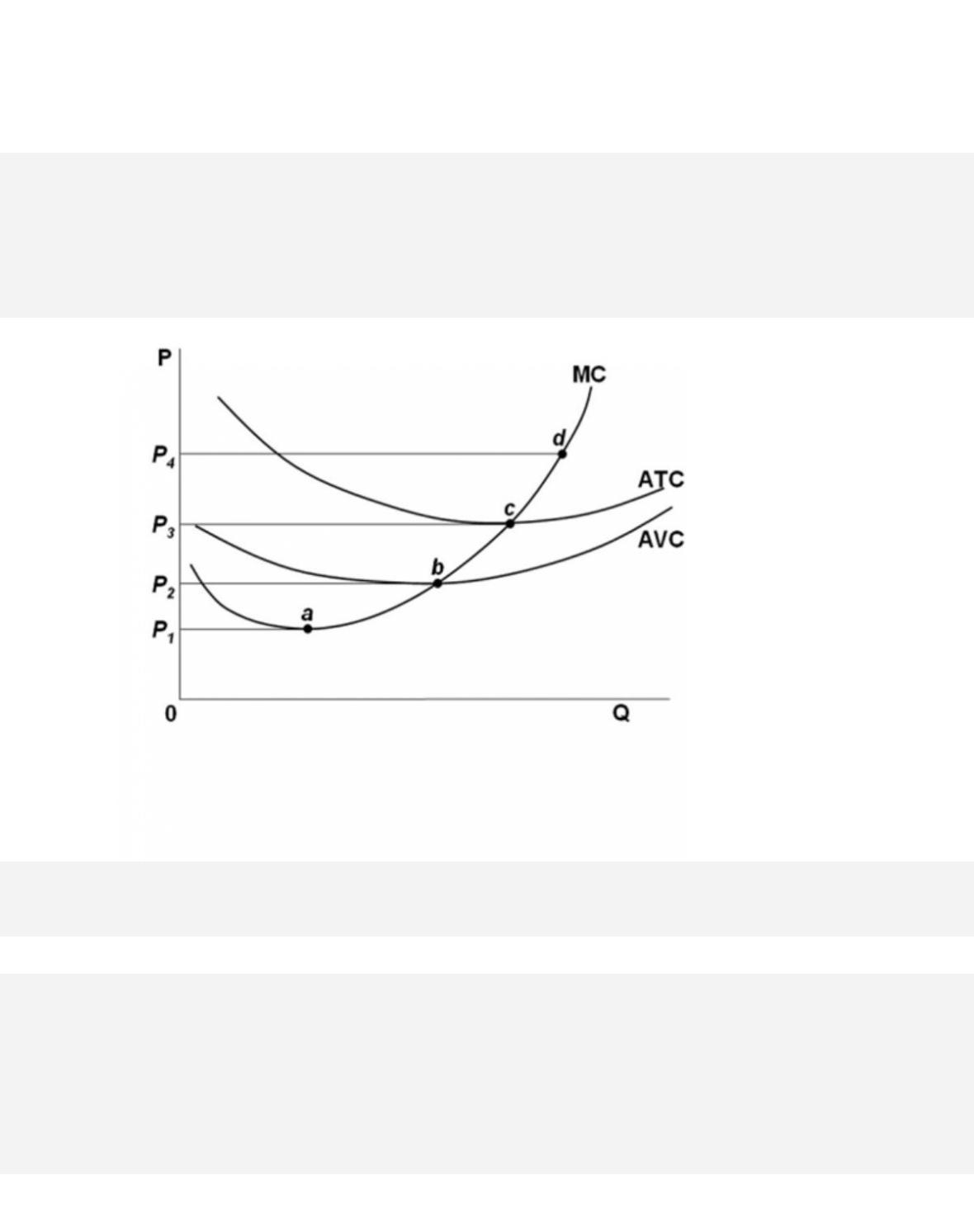
Refer to the diagram for a purely competitive producer. The firm’s short-run supply curve is
67.
The short-run supply curve of a purely competitive producer is based primarily on its

10–34
Copyright © 2018 McGraw-Hill Education. All rights reserved. No reproduction or distribution without the prior
written consent of McGraw-Hill Education.
D. MC curve.
68.
On a per-unit basis, economic profit can be determined as the difference between
69.
In the short run, a purely competitive seller will shut down if

70.
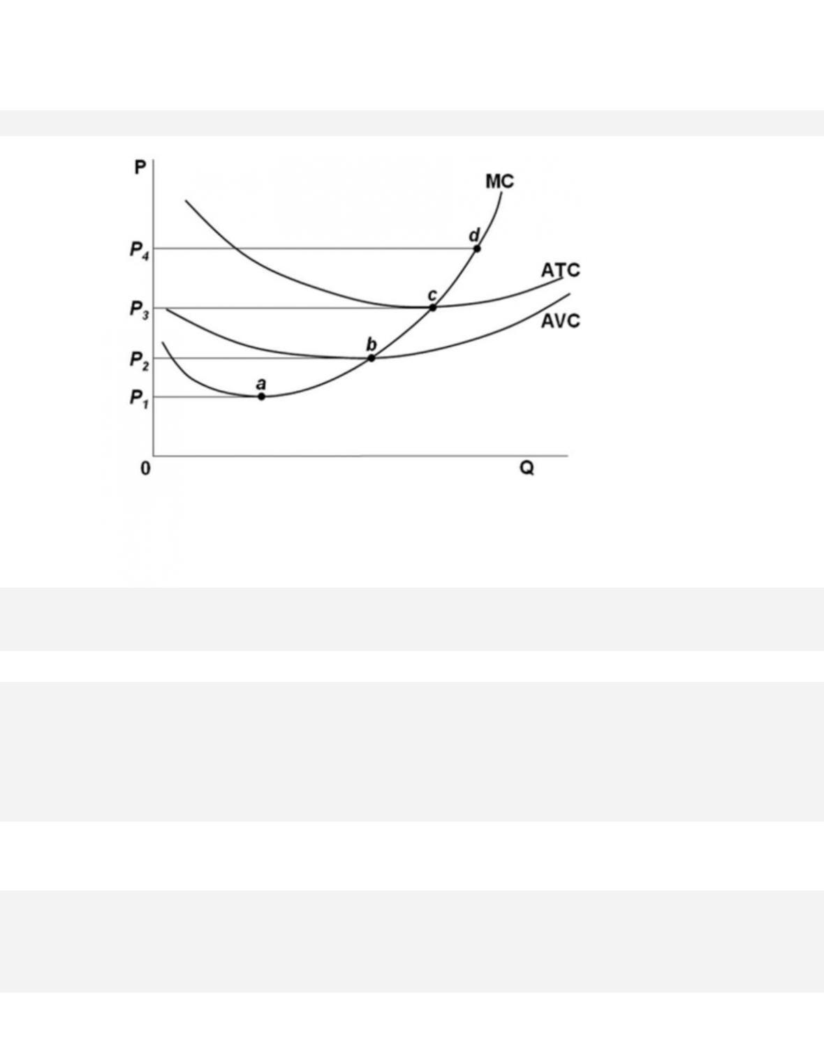
According to the accompanying diagram, to maximize profit or minimize losses, this firm will
produce
71.
Refer to the accompanying diagram. At the profit-maximizing output, total revenue will be
72.
According to the accompanying diagram, at the profit-maximizing output, total fixed cost is
equal to
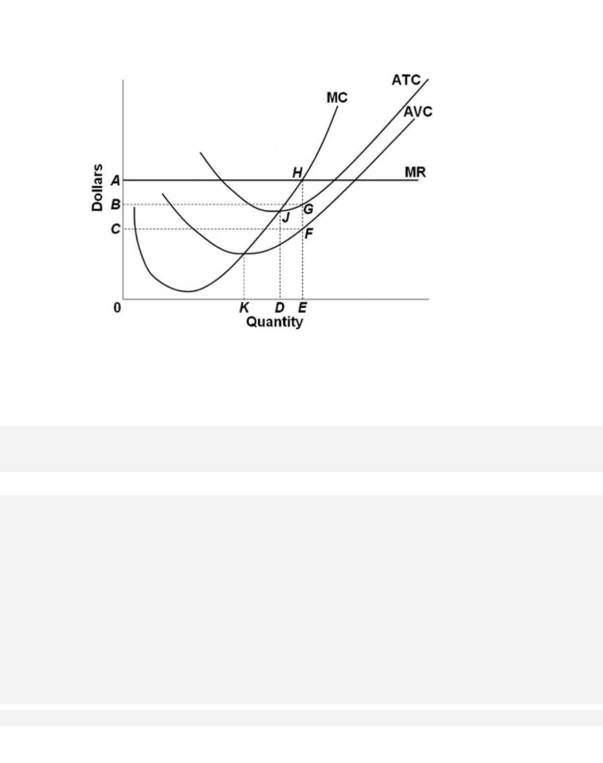
73.
According to the accompanying diagram, at the profit-maximizing output, total variable cost is
equal to
74.
According to the accompanying diagram, at the profit-maximizing output, the firm will realize
75. If a purely competitive firm is producing at some output level less than the profit-
maximizing output, then
10–40
Copyright © 2018 McGraw-Hill Education. All rights reserved. No reproduction or distribution without the prior
written consent of McGraw-Hill Education.
D. marginal revenue exceeds marginal cost.
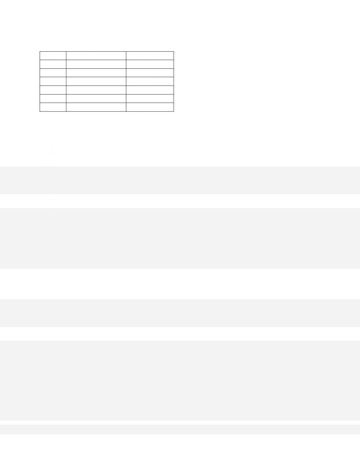
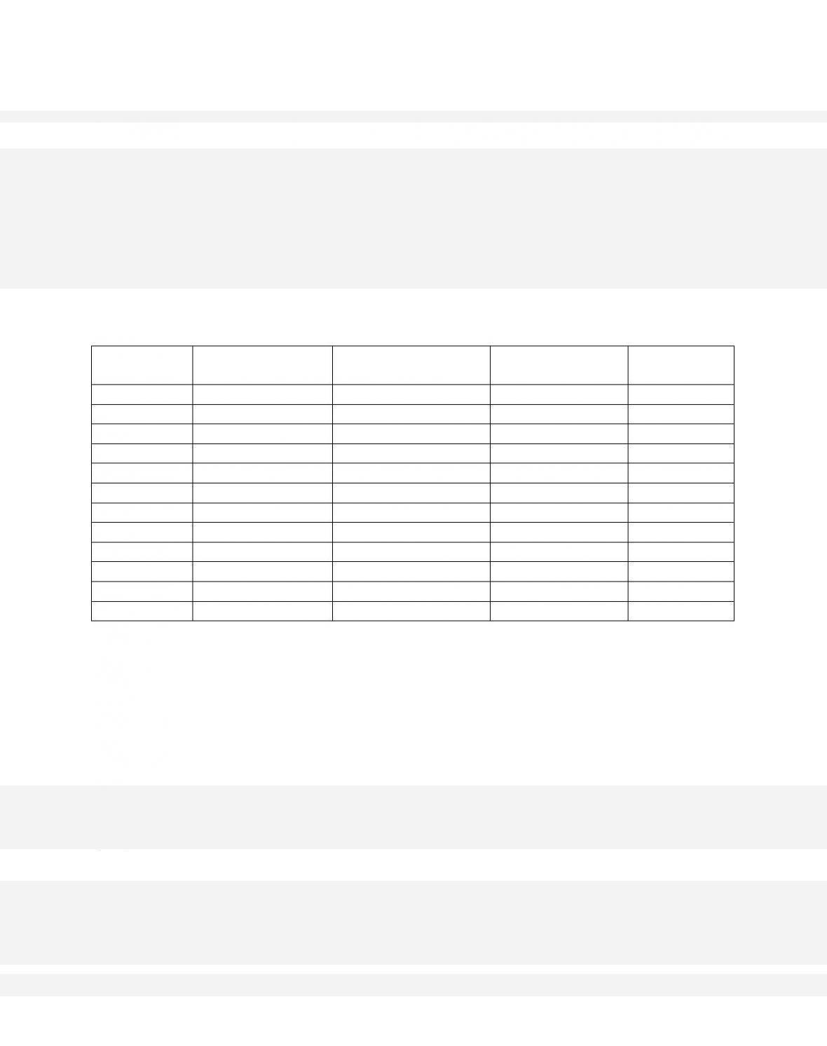
76.
Total
Product
Average Fixed
Cost
Average Variable
Cost
Average Total
Cost
Marginal
Cost
1
$100.00
$17.00
$117.00
$17
2
50.00
16.00
66.00
15
3
33.33
15.00
48.33
13
4
25.00
14.25
39.25
12
5
20.00
14.00
34.00
13
6
16.67
14.00
30.67
14
7
14.29
15.71
30.00
26
8
12.50
17.50
30.00
30
9
11.11
19.44
30.55
35
10
10.00
21.60
31.60
41
11
9.09
24.00
33.09
48
12
8.33
26.67
35.00
56
The accompanying table gives cost data for a firm that is selling in a purely competitive market.
If the market price for the firm‘s product is $12, the
competitive firm should produce