CHAPTER 38
Extending the Analysis of Aggregate Supply
A. Short-Answer, Essays, and Problems
1. John Maynard Keynes stated that “In the long run we are all dead!” Explain what he meant by this.
2. What is the basic difference between the short run and long run as these terms relate to macroeconomics?
Why does this difference occur?
3. Describe the characteristics of the short-run aggregate supply curve. Explain what happens to: (1) nominal
wages; (2) employment; (3) output; (4) revenues; and, (5) profits as the price level increases from the full-
4. Suppose the potential level of real domestic output (Q) for a hypothetical economy is $250 and the price
level (P) initially is 100. Use the following short-run aggregate supply schedules below to answer the
questions.
AS (P = 100)
AS (P = 110)
AS (P = 90)
P
Q
P
Q
P
Q
110
280
110
250
110
310
100
250
100
220
100
280
90
220
90
190
90
250
5. Suppose the potential level of real domestic output (Q) for a hypothetical economy is $160 and the price
level (P) initially is 200. Use the following short-run aggregate supply schedules to answer the questions.
AS (P = 200)
AS (P = 210)
AS (P = 190)
P
Q
P
Q
P
Q
210
190
210
160
210
220
200
160
200
130
200
190
190
130
190
100
190
160

38-749
Copyright © 2017 McGraw-Hill Education. All rights reserved. No reproduction or distribution without the prior written consent
of McGraw-Hill Education.
(b) What will be the long-run level of real GDP when the price level rises from 200 to 210? Falls from
200 to 190? Explain each situation.
6. Explain the reasoning behind why the long-run aggregate supply curve is vertical.
7. Describe the characteristics of the long-run aggregate supply curve. Explain how changes in the price level
8. What is the long-run equilibrium in the extended aggregate demand and aggregate supply model?
9. Describe the process that occurs with demand-pull inflation in the extended aggregate demand and
10. Describe cost-push inflation in the extended aggregate demand and aggregate supply model. Explain the
policy dilemma for government policy if they take no action or use monetary and fiscal policy to counter
11. Differentiate between “demand–pull” and “cost–push” inflation in the basic aggregate demand and
12. Explain what happens in the extended aggregate demand and aggregate supply model when there is a
13. Use the extended AD–AS model to explain how inflation depends on aggregate demand and not the level
14. How do modern economies experience ongoing inflation when achieving economic growth?
15. How would economic growth be shown in a production possibilities graph and in a graph of long-run
aggregate supply?
16. How would economic growth and mild inflation be depicted in the extended aggregate demand and
aggregate supply model?
17. What are three significant generalizations supported by results from the extended AD-AS model?
18. What is the Phillips Curve? What concept does it illustrate?
19. Explain the Phillips Curve concept and construct an example of the curve on the below graph.
20. If the Phillips Curve exists in reality, what dilemma does this create for fiscal and monetary policies?
21. What is stagflation and what was one of its causes in the 1970s and early 1980s?

38-750
38-751
22. Assume the following information is relevant for an advanced economy over a three-year period. Describe
in detail the macroeconomic situation faced by this society. Is cost-push inflation evident? What
corrective policies would you recommend and why?
Year
Price
index
Increase in
labor
productivity
Increase in
industrial
production
Unemp.
Rate
Average
hourly
wage
1
167
4%
4%
4.5%
$6.00
2
174
3
2
5.2
6.50
3
181
2.5
1.5
5.8
7.10
23. What contributed to stagflation’s demise between 1982 and 1989? How did these events affect aggregate
supply and the Phillips Curve?
24. What economic events and policies led to the emergence of the U.S. economy from the stagflation of the
25. Discuss the shifts to the Phillips curve that occurred during and after the financial crisis. Was this
consistent with a stable curve?
26. Evaluate the misery index and its effectiveness during a recession.
27. What is the misery index? Why do economists find it to be a flawed measure?
28. Compare and contrast the short-run Phillips Curve and the long-run Phillips Curve.
29. Discuss, using the Philips Curve, the effect of a policy aimed at lowering the inflation rate.
30. Answer the questions based on the following diagram.
31. Why is the difference between the actual and expected rates of inflation important for explaining inflation?
32. What is disinflation? Give examples of it.
33. Why is the difference between the actual and expected rates of inflation important for explaining
disinflation?
38-752
35. How do supply-side economists see reducing taxes as a way to improve productivity?
39. Use the following diagram to answer the next three questions.
40. Draw a Laffer Curve and explain the relationship it purports to portray. Why might this curve be important
for macroeconomic policy?
41. Suppose an the government has a current tax rate of c. Knowing the Laffer Curve is depicted below advise
the president on whether the tax rate should be increased, decreased, or remain the same.

42. (Consider This) How did Arthur Laffer use Robin Hood and Sherwood Forest to explain the advantage of
supply-side economics?
43. What is supply-side economics? What is the rationale for it? Is it effective?
44. What are the major criticisms of the Laffer Curve and supply-side economics?
45. How do supply-side advocates respond to critics? How valid is their defense?
46. (Last Word) Do tax increases reduce real GDP?

38-754
B. Answers to Short-Answer, Essays, and Problems
1. John Maynard Keynes stated that “In the long run we are all dead!” Explain what he meant by this.
2. What is the basic difference between the short run and long run as these terms relate to macroeconomics?
Why does this difference occur?
3. Describe the characteristics of the short-run aggregate supply curve. Explain what happens to: (1) nominal
wages; (2) employment; (3) output; (4) revenues; and, (5) profits as the price level increases from the full-
employment level of output. Then explain what happens to these variables as the price level decreases
from the full-employment-level of output.
The short-run aggregate supply curve will be an upsloping curve with the price level on the vertical axis

38-755
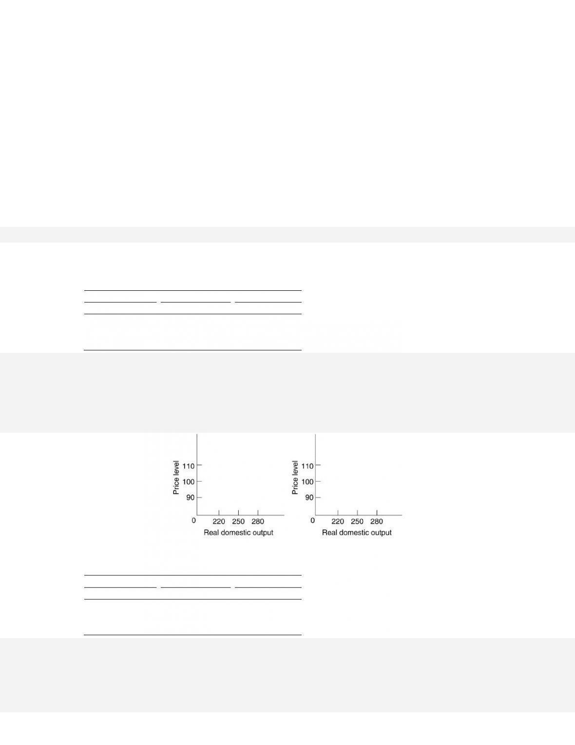
4. Suppose the potential level of real domestic output (Q) for a hypothetical economy is $250 and the price
level (P) initially is 100. Use the following short-run aggregate supply schedules below to answer the
questions.
AS (P = 100)
AS (P = 110)
AS (P = 90)
P
Q
P
Q
P
Q
110
280
110
250
110
310
100
250
100
220
100
280
90
220
90
190
90
250
(a) What will be the short-run level of real GDP if the price level rises unexpectedly from 100 to 110
because of an increase in aggregate demand? Falls unexpectedly from 100 to 90 because of a decrease
in aggregate demand? Explain each situation.
(b) What will be the long-run level of real GDP when the price level rises from 100 to 110? Falls from
100 to 90? Explain each situation.
(c) Show the circumstances described in (a) and (b) on the graph below and derive the long-run aggregate
supply curve.
(a) In the short run, the table reports that real GDP will rise to 280 when the price level rises from 100 to

38-756
5. Suppose the potential level of real domestic output (Q) for a hypothetical economy is $160 and the price
level (P) initially is 200. Use the following short-run aggregate supply schedules to answer the questions.
AS (P = 200)
AS (P = 210)
AS (P = 190)
P
Q
P
Q
P
Q
210
190
210
160
210
220
200
160
200
130
200
190
190
130
190
100
190
160
(a) What will be the short-run level of real GDP if the price level rises unexpectedly from 200 to 210
because of an increase in aggregate demand? Falls unexpectedly from 200 to 190 because of a
decrease in aggregate demand? Explain each situation.
(b) What will be the long-run level of real GDP when the price level rises from 200 to 210? Falls from
200 to 190? Explain each situation.
6. Explain the reasoning behind why the long-run aggregate supply curve is vertical.
7. Describe the characteristics of the long-run aggregate supply curve. Explain how changes in the price level
affect the short-run aggregate supply curve and the long-run aggregate supply curve.
The long-run aggregate supply curve will be vertical at the full-employment level of output. Changes in

38-757
8. What is the long-run equilibrium in the extended aggregate demand and aggregate supply model?
9. Describe the process that occurs with demand-pull inflation in the extended aggregate demand and
aggregate supply model.
10. Describe cost-push inflation in the extended aggregate demand and aggregate supply model. Explain the
policy dilemma for government policy if they take no action or use monetary and fiscal policy to counter
the cost-push inflation.
Assume that the economy is initially in equilibrium at the full-employment level of real output. Also
assume that there is a major increase in the price of a major resource (e.g., oil) for the economy. In this
11. Differentiate between “demand–pull” and “cost–push” inflation in the basic aggregate demand and
aggregate supply model.

12. Explain what happens in the extended aggregate demand and aggregate supply model when there is a
recession.
13. Use the extended AD–AS model to explain how inflation depends on aggregate demand and not the level
of real GDP.
14. How do modern economies experience ongoing inflation when achieving economic growth?
15. How would economic growth be shown in a production possibilities graph and in a graph of long-run
aggregate supply?
16. How would economic growth and mild inflation be depicted in the extended aggregate demand and
aggregate supply model?
17. What are three significant generalizations supported by results from the extended AD-AS model?
38-759
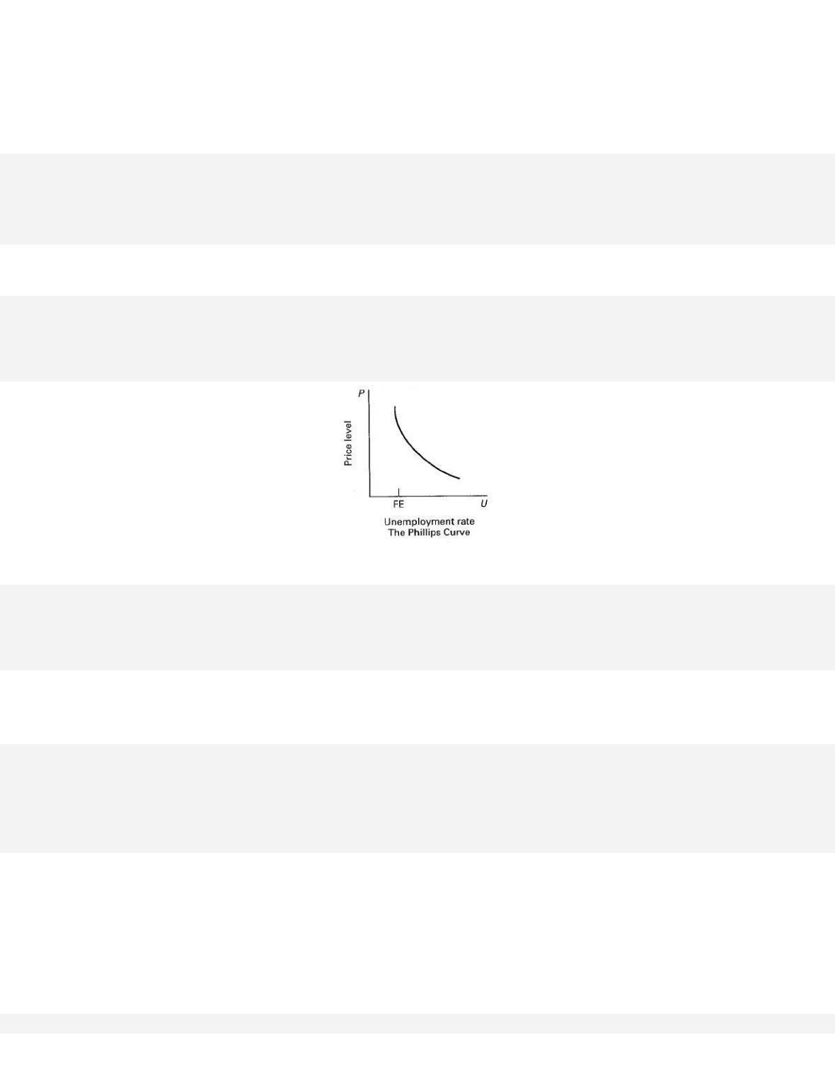
18. What is the Phillips Curve? What concept does it illustrate?
The Phillips Curve shows the relationship between the unemployment rate and the rate of inflation. The
19. Explain the Phillips Curve concept and construct an example of the curve on the below graph.
20. If the Phillips Curve exists in reality, what dilemma does this create for fiscal and monetary policies?
21. What is stagflation and what was one of its causes in the 1970s and early 1980s?
Stagflation is the presence of both inflation and unemployment over a period of time such as occurred in

22. Assume the following information is relevant for an advanced economy over a three-year period. Describe
in detail the macroeconomic situation faced by this society. Is cost-push inflation evident? What
corrective policies would you recommend and why?
Year
Price
index
Increase in
labor
productivity
Increase in
industrial
production
Unemp.
Rate
Average
hourly
wage
1
167
4%
4%
4.5%
$6.00
2
174
3
2
5.2
6.50
3
181
2.5
1.5
5.8
7.10
This economy seems to be in a period of stagflation—inflation is rising at the same time that
unemployment is increasing. There appear to be two reasons for this: labor productivity and industrial
production growth are falling, and at the same time the hourly wage rate is rising. This indicates an
increase in unit labor costs that must be covered by rising prices or firms will cut back still further on
output plans due to declining profits, which would be caused by the increase in labor cost, and decline in
production. Cost-push inflation is present.
23. What contributed to stagflation’s demise between 1982 and 1989? How did these events affect aggregate
supply and the Phillips Curve?
24. What economic events and policies led to the emergence of the U.S. economy from the stagflation of the
late 1970s and early 1980s? Depict the effect of these events using the extended AD–AS model.
25. Discuss the shifts to the Phillips curve that occurred during and after the financial crisis. Was this consistent
with a stable curve?

26. Evaluate the misery index and its effectiveness during a recession.
27. What is the misery index? Why do economists find it to be a flawed measure?
28. Compare and contrast the short-run Phillips Curve and the long-run Phillips Curve.
29. Discuss, using the Philips Curve, the effect of a policy aimed at lowering the inflation rate.
When policy makers decide the inflation rate is too high and needs to be lowered it will not only influence
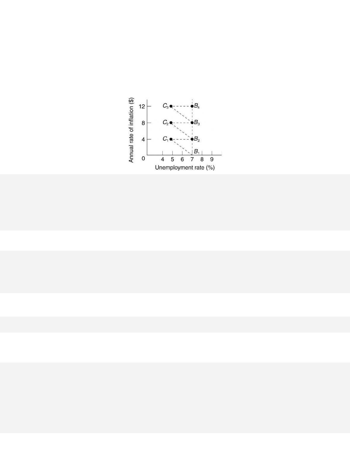
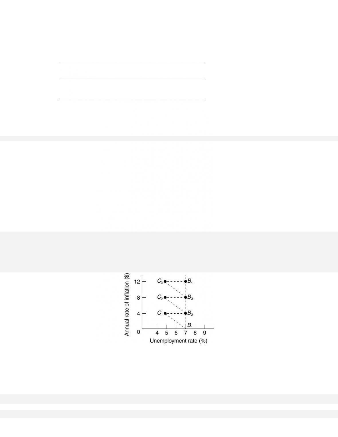
30. Answer the questions based on the following diagram.
(a) Assume the economy is initially at point B1 and there is an increase in aggregate demand which results
in a 4% increase in prices. Describe the short-run and long-run outcomes that would result in this
economy.
(b) Assume the economy is initially at point B2, and there is an increase in aggregate demand. What will
happen in the economy? Explain, using the graph.
(c) Based on this diagram, what would the prediction be for the natural (full-employment) rate of
unemployment?
(a) In the short run, the unemployment rate will fall to C1, or 5% from its original level of 7% as firms
31. Why is the difference between the actual and expected rates of inflation important for explaining inflation?
32. What is disinflation? Give examples of it.
33. Why is the difference between the actual and expected rates of inflation important for explaining
disinflation?

38-763
38-764
34. “Lower prices are always good for business.” Evaluate this statement.
This statement is incorrect. Lower prices are not necessarily good for business. In the long run, the level
of prices is irrelevant as wages adjust to compensate for price levels, maintaining workers’ purchasing
power and the firms’ profits.
35. How do supply-side economists see reducing taxes as a way to improve productivity?
36. Explain the basic arguments for supply-side economics.
37. Contrast “supply–side” economics with “demand–side” fiscal policy.
38. What is the Laffer Curve? Explain the relationship that is shown in the curve.
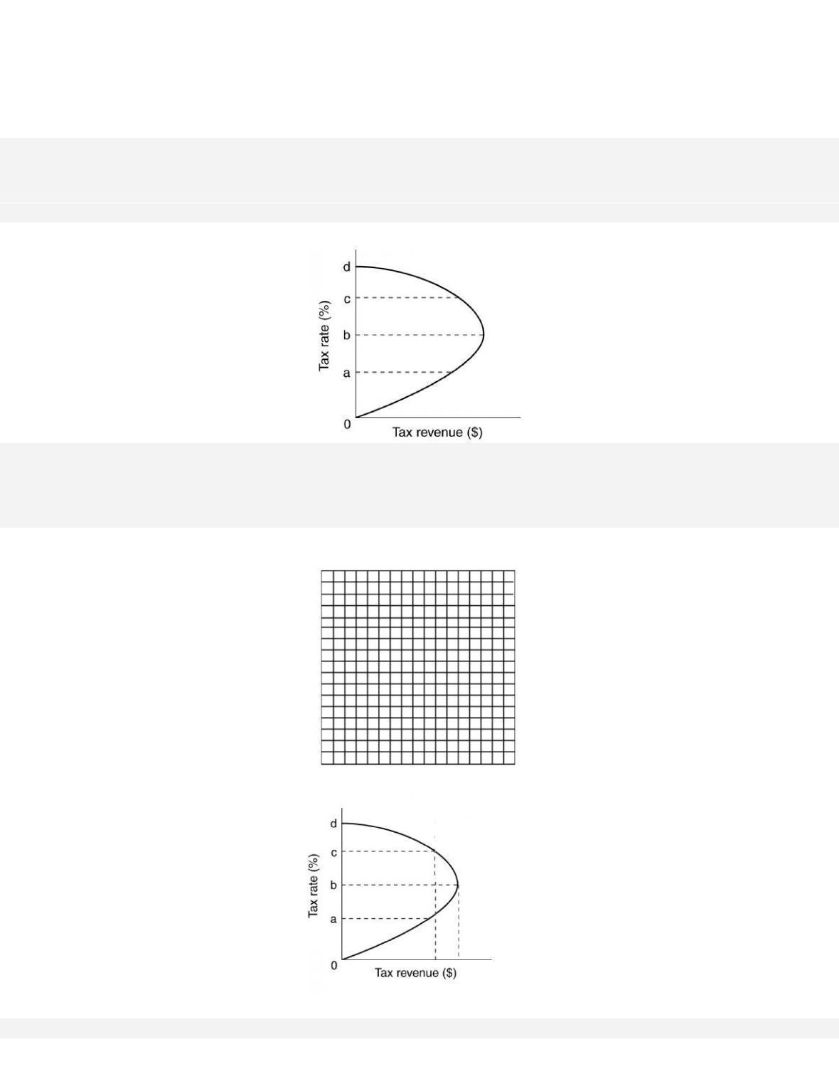
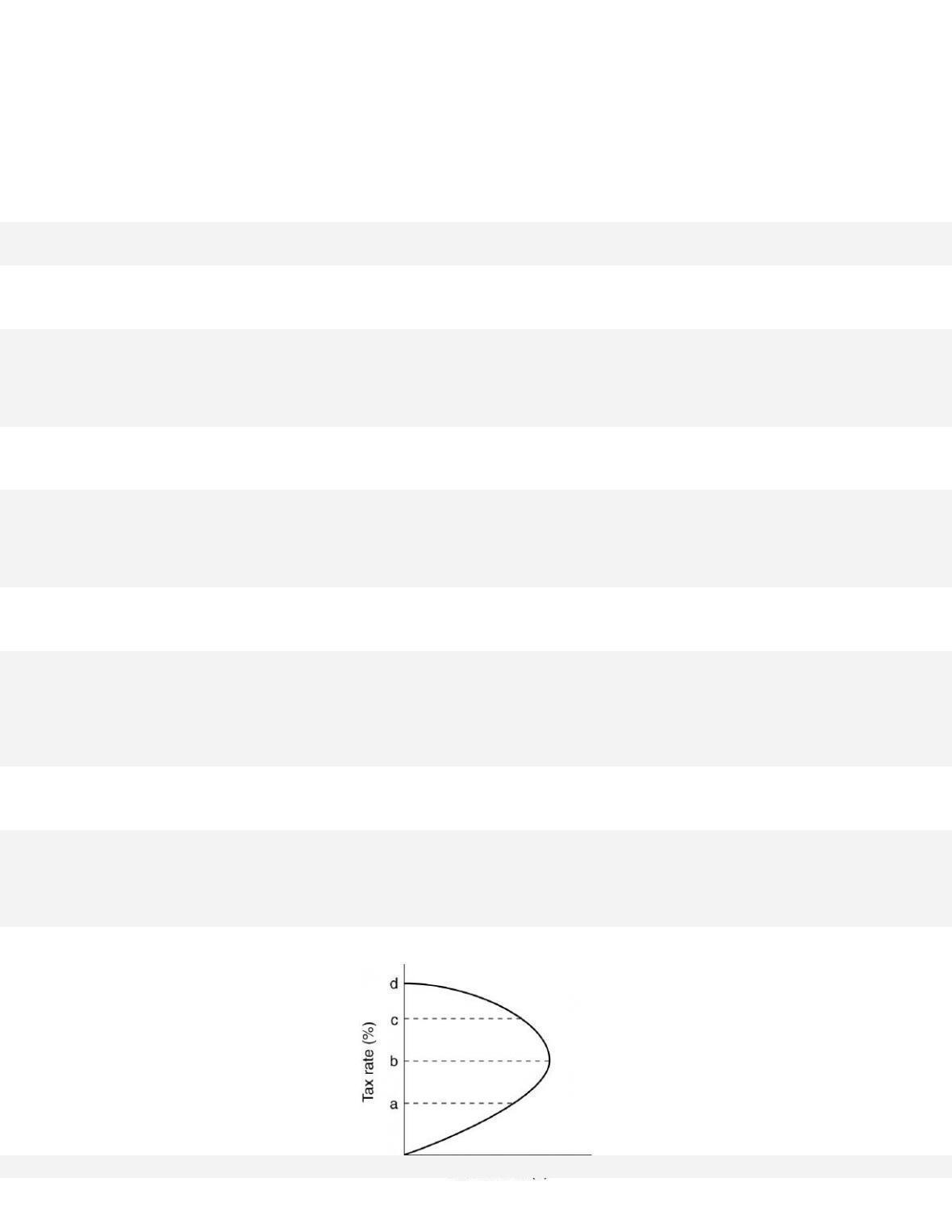
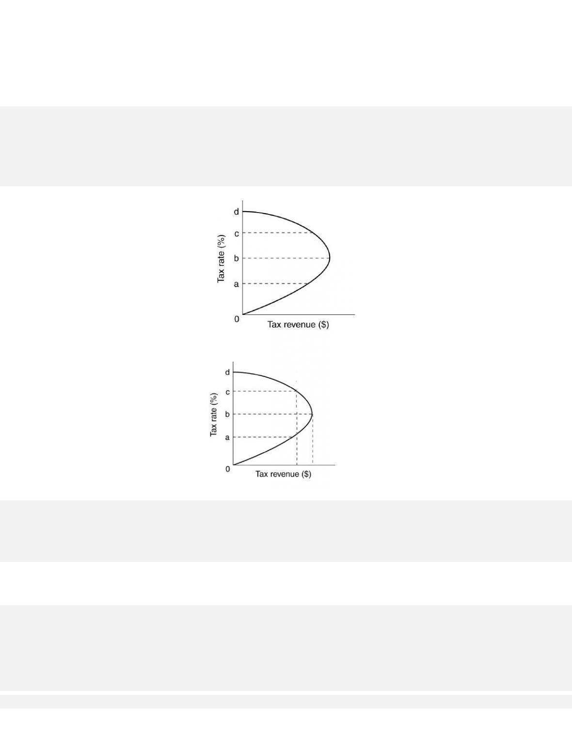
39. Use the following diagram to answer the next three questions.

38-765
(a) What is this diagram called and what does it say about the relationship between tax rates and tax
revenues?
(b) If tax rates are at level c, should the government raise or lower tax rates to increase revenues? Explain.
(c) What does tax level b represent? Could policy makers find the actual rate that b represents? Discuss
this point.
40. Draw a Laffer Curve and explain the relationship it purports to portray. Why might this curve be important
for macroeconomic policy?
41. Suppose an the government has a current tax rate of c. Knowing the Laffer Curve is depicted below advise
the president on whether the tax rate should be increased, decreased, or remain the same.
As an advisor to the president, you should recommend that the tax rate be reduced for two reasons. First,
42. (Consider This) How did Arthur Laffer use Robin Hood and Sherwood Forest to explain the advantage of
supply-side economics?

43. What is supply-side economics? What is the rationale for it? Is it effective?
44. What are the major criticisms of the Laffer Curve and supply-side economics?
45. How do supply-side advocates respond to critics? How valid is their defense?
46. (Last Word) Do tax increases reduce real GDP?