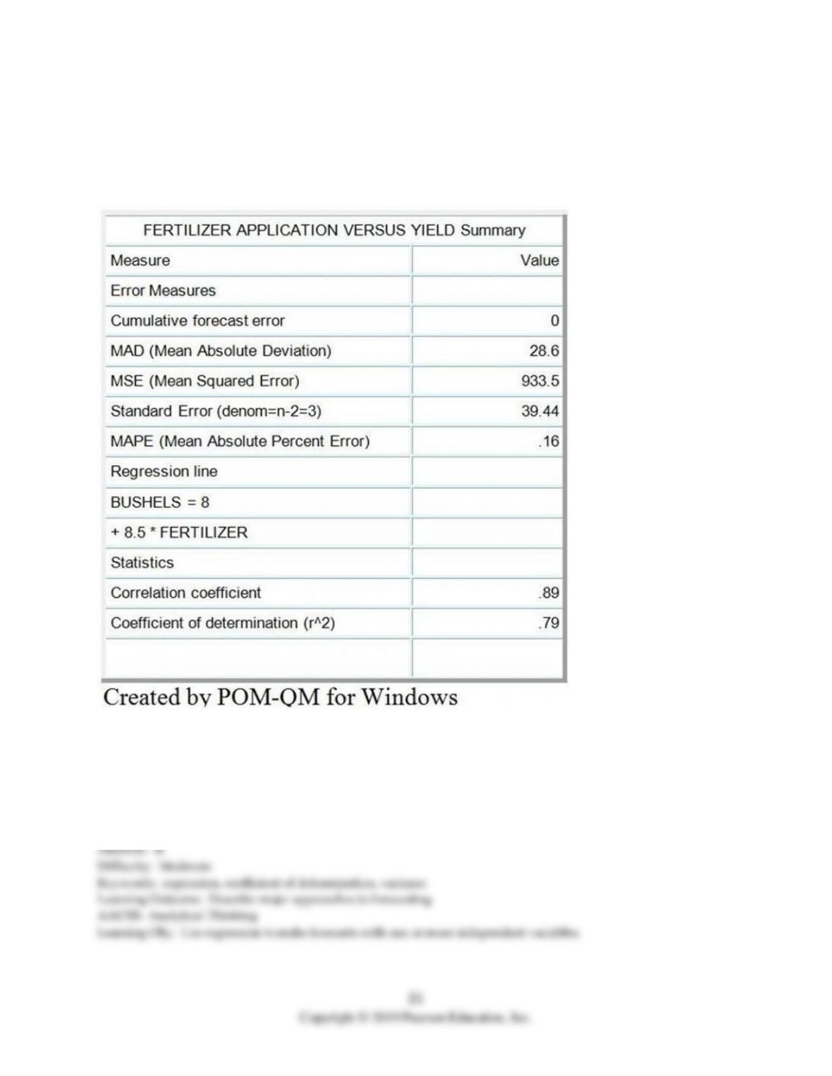
Table 8.2
The Agricultural Extension Agent’s Office has tracked fertilizer application and crop yields for a variety
of chickpea and has recorded the data shown in the following table. Their staff statistician developed the
regression model and computed the performance statistics displayed below the data.
6) Use the information provided in Table 8.2. What percent in the variation of the variable Bushels is
explained by the value of the variable Fertilizer?
A) 89%
B) 79%
C) 71%
D) 50%
7) Use the information provided in Table 8.2. For every unit of fertilizer applied, the crop yield increases
by:
A) 8.0 bushels.
B) 8.5 bushels.
C) 8.9 bushels.
D) 7.9 bushels.
8) Use the information provided in Table 8.2. The value of Bushels when Fertilizer is 60 is:
A) 2520.
B) 490.
C) 390.
D) 518.
9) Use the information provided in Table 8.2. The value of Fertilizer required to generate 100 bushels yield
must be:
A) 10.82.
B) 12.25.
C) 10.26.
D) 9.07.
10) Use the information in Table 8.2. If the correlation coefficient were negative, which of these statements
would be true?
A) The coefficient of determination would also be negative.
B) An increase in fertilizer would result in a decrease in crop yield.
C) Applying no fertilizer would mean a negative crop yield.
D) The standard error would also be negative.
23
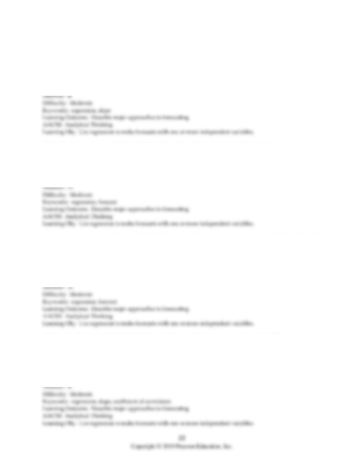
Table 8.3
A textbook publisher for books used in business schools believes that the number of books sold is related
to the number of campus visits to decision makers made by their sales force. A sampling of the number of
sales calls made and the number of books sold is shown in the following table.
NUMBER OF SALES
CALLS MADE
NUMBER OF BOOKS
SOLD
25
375
15
250
25
525
45
825
35
550
25
575
25
550
35
575
25
400
15
400

11) Use the information provided in Table 8.3. What percent in the variation of the variable Books Sold is
explained by the value of the variable Sales Calls Made?
A) 86.5%
B) 83.3%
C) 74.8%
D) 72.5%
12) Use the information provided in Table 8.3. For every sale call made, the number of books sold
increases by:
A) 14.74 books.
B) 104.6 books.
C) 83.30 books.
D) 7.25 books.
13) Use the information provided in Table 8.3. If a sales representative makes 55 sales calls, the number of
book sales the publisher should expect is:
A) 105.
B) 4,581.
C) 114.
D) 915.

25
14) Use the information provided in Table 8.3. In order to realize the sale of 700 books, how many sales
calls will the sales representative have to make?
A) 40.4
B) 45.9
C) 32.7
D) 37.6
Table 8.4
The Furniture Super Mart is a furniture retailer in Evansville, Indiana. The Marketing Manager wants to
prepare a media budget based on the next quarter’s business plan. The manager wants to decide the mix
of radio advertising and newspaper advertising needed to generate varying levels of Weekly Gross
Revenue. The manager has collected data for the past five weeks, and has recorded the following average
Weekly Gross Revenues and expenditures for Weekly Radio (X1) and Newspaper (X2) advertising:
WEEK
AVERAGE
WEEKLY GROSS
REVENUE ($000)
AVERAGE
WEEKLY RADIO
ADVERTISING
($000)
AVERAGE
WEEKLY
NEWSPAPER
ADVERTISING
($000)
1
60
6
1
2
45
3
3
3
55
4
2
4
70
5
3
5
40
2
1
The Manager uses the multiple regression model in OM Explorer and obtains the following results:
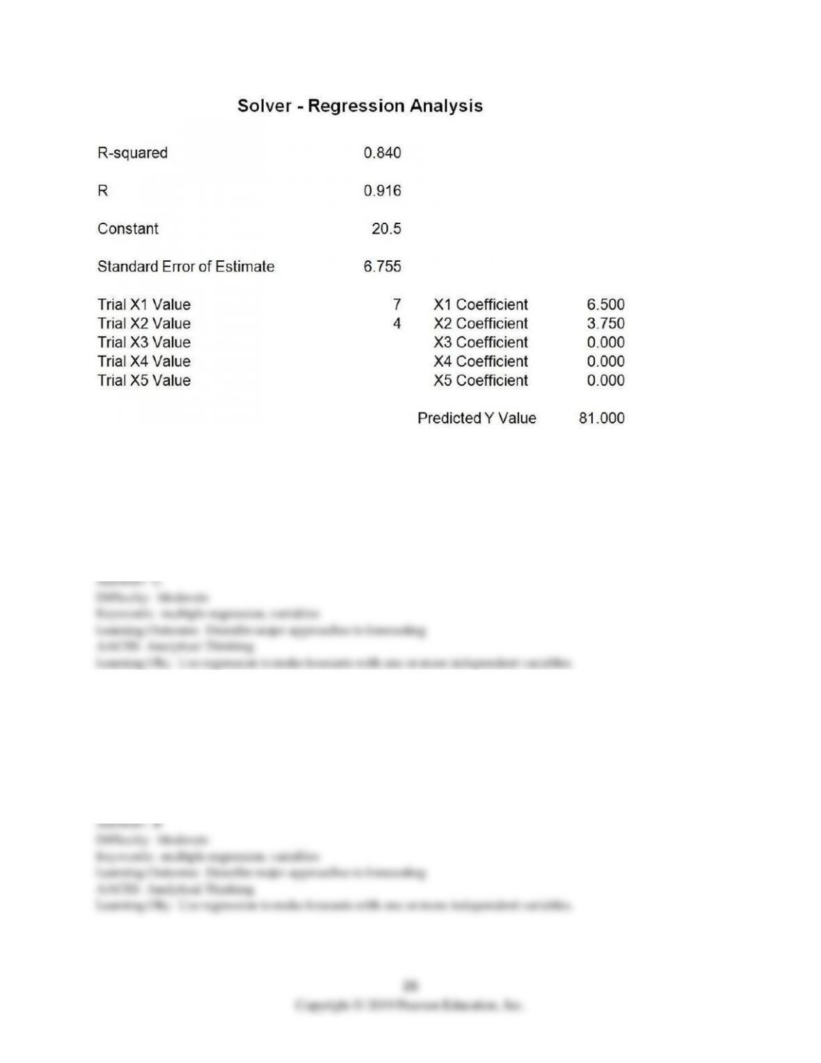
15) Use the information provided in Table 8.4. Adding $1,000 of Weekly Radio Advertising (X1) can be
expected to increase Weekly Gross Revenues by what amount? (Assume all other variables are held
constant.)
A) $20,500
B) $3,750
C) $6,500
D) $10,250
16) Use the information provided in Table 8.4. Adding $1,000 of Weekly Newspaper Advertising (X2) can
be expected to increase Weekly Gross Revenues by what amount? (Assume all other variables are held
constant.)
A) $20,500
B) $3,750
C) $6,500
D) $10,250
17) Use the information provided in Table 8.4. What amount of Weekly Gross Revenue can be expected
for a week in which no radio or newspaper advertising is purchased? (Assume all other variables are held
constant.)
A) $20,500
B) $3,750
C) $6,500
D) $10,250
18) Use the information provided in Table 8.4. What is the estimated Weekly Gross Revenue if $7,000 is
spent on Radio Advertising (X1) and $4,000 is spent on Newspaper Advertising (X2)?
A) $45,500
B) $15,000
C) $60,500
D) $81,000
19) Use the information provided in Table 8.4. What is the estimated Weekly Gross Revenue if $4,000 is
spent on Radio Advertising (X1) and $7,000 is spent on Newspaper Advertising (X2)?
A) $52,250
B) $26,250
C) $72,750
D) $20,500
20) Which one of the following is an example of causal forecasting technique?
A) weighted moving average
B) linear regression
C) exponential smoothing
D) Delphi method
21) ________ is a causal method of forecasting in which one variable is related to one or more variables by
a linear equation.
22) The ________ variable is the variable that one wants to forecast.
23) ________ are assumed to “cause” the results that a forecaster wishes to predict.
24) A(n) ________ measures the direction and strength between the independent variable and the
dependent variable.
29
25) The ________ measures the amount of variation in the dependent variable about its mean that is
explained by the regression line.
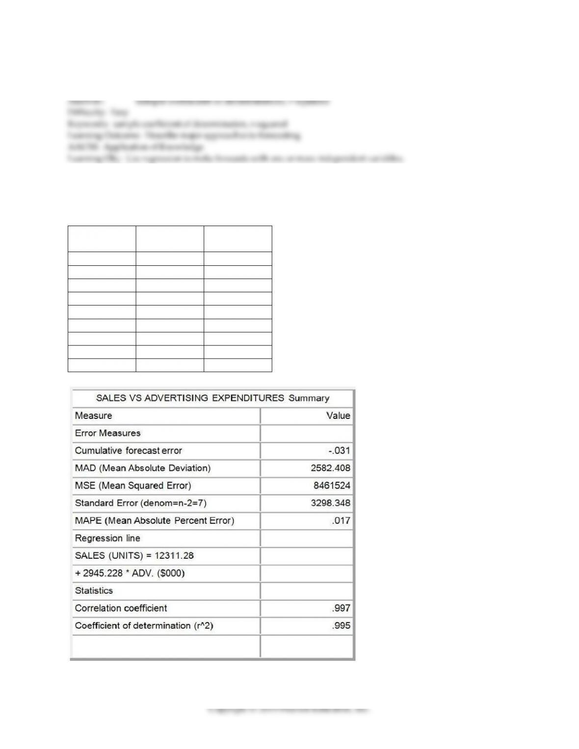
26) The marketing department for a major manufacturer tracks sales and advertising expenditures each
month. Data from the past nine months and regression output appear in the following table. Interpret the
equation coefficients and the values for the coefficient of determination and the correlation coefficient.
Month
Sales (units)
Advertising
($1,000)
1
86,010
25
2
134,697
40
3
202,025
65
4
141,180
45
5
217,086
70
6
178,399
55
7
156,975
50
8
113,155
35
9
191,901
60
Created by POM-QM for Windows
30
Copyright © 2019 Pearson Education, Inc.
Answer: The regression equation is:
Y = a + bX
Sales (units) = 12,311.28 + 2,945.23 × Advertising ($ in 000s)
The intercept of 12,311 suggests that if no money were spent on advertising, sales would be 12,311 units
for that month. The slope may be interpreted as for every $1,000 spent on advertising, sales increase by a
little over 2,945 units.
The correlation coefficient of 0.997 shows a very strong positive relationship between the independent
and dependent variables. The sample coefficient of determination is 0.995, so the level of advertising
expenditure explains 99.5% of the variation in sales.
Difficulty: Moderate
Keywords: regression, correlation coefficient, coefficient of determination
Learning Outcome: Describe major approaches to forecasting
AACSB: Analytical Thinking
Learning Obj.: Use regression to make forecasts with one or more independent variables.
8.6 Time-Series Methods
1) Time-series analysis is a statistical approach that relies heavily on historical demand data to project the
future size of demand.
2) The naive forecast may be adapted to take into account a demand trend.
3) A naive forecast is a time-series method whereby the forecast for the next period equals the demand
for the current period.
4) A simple moving average of one period will yield identical results to a naive forecast.
5) An exponential smoothing model with an alpha equal to 1.00 is the same as a naive forecasting model.
6) The trend projection with regression model can forecast demand well into the future.
7) Which one of the following statements about forecasting is false?
A) You should use the simple moving-average method to estimate the mean demand of a time series that
has a pronounced trend and seasonal influences.
B) The weighted moving-average method allows forecasters to emphasize recent demand over earlier
demand. The forecast will be more responsive to change in the underlying average of the demand series.
C) The most frequently used time-series forecasting method is exponential smoothing because of its
simplicity and the small amount of data needed to support it.
D) In exponential smoothing, higher values of alpha place greater weight on recent demands in
computing the average.
8) When the underlying mean of a time series is very stable and there are no trend, cyclical, or seasonal
influences:
A) a simple moving-average forecast with n = 20 should outperform a simple moving-average forecast
with n = 3.
B) a simple moving-average forecast with n = 3 should outperform a simple moving-average forecast with
n = 15.
C) a simple moving-average forecast with n = 20 should perform about the same as a simple moving-
average forecast with n = 3.
D) an exponential smoothing forecast with a = 0.30 should outperform a simple moving-average forecast
with α = 0.01.
9) With the multiplicative seasonal method of forecasting:
A) the times series cannot exhibit a trend.
B) seasonal factors are multiplied by an estimate of average demand to arrive at a seasonal forecast.
C) the seasonal amplitude is a constant, regardless of the magnitude of average demand.
D) there can be only four seasons in the time-series data.
10) Which one of the following statements about forecasting is false?
A) The method for incorporating a trend into an exponentially smoothed forecast requires the estimation
of three smoothing constants: one for the mean, one for the trend, and one for the error.
B) The cumulative sum of forecast errors (CFE) is useful in measuring the bias in a forecast.
C) The standard deviation and the mean absolute deviation measure the dispersion of forecast errors.
D) A tracking signal is a measure that indicates whether a method of forecasting has any built-in biases
over a period of time.
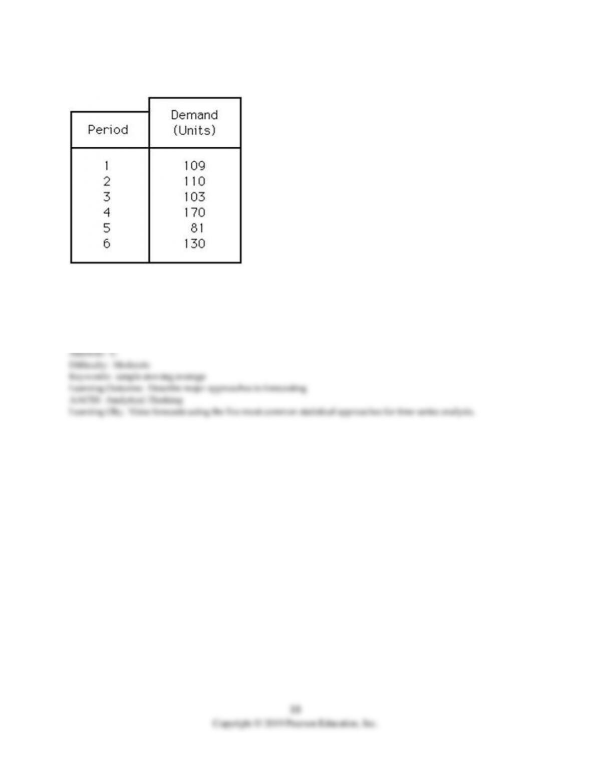
11) Demand for a new five-inch color TV during the last six periods has been as follows:
What is the forecast for period 7 if the company uses the simple moving-average method with n = 4?
A) fewer than or equal to 115
B) greater than 115 but fewer than or equal to 120
C) greater than 120 but fewer than or equal to 125
D) greater than 125
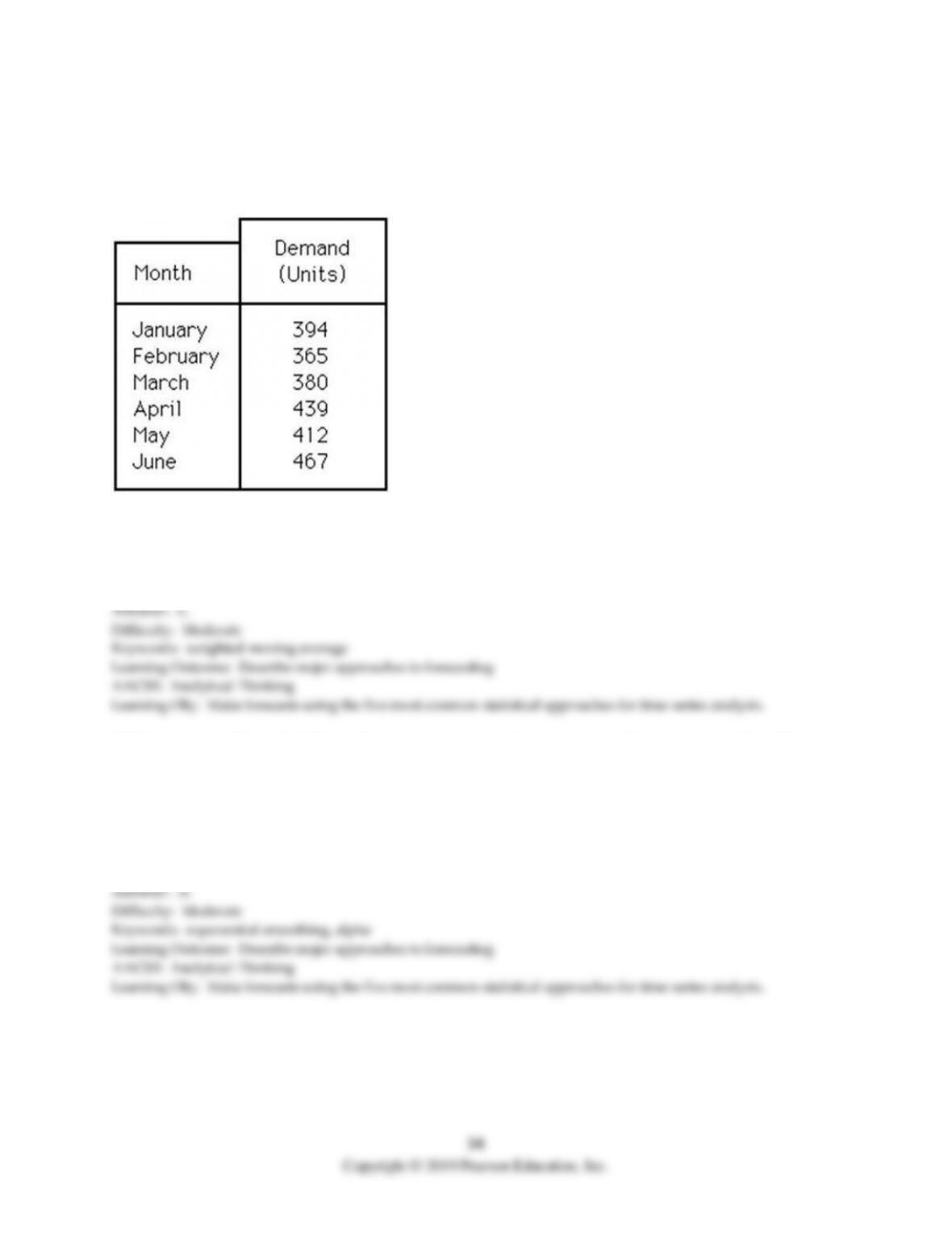
12) Demands for a newly developed salad bar at the Great Professional restaurant for the first six months
of this year are shown in the following table. What is the forecast for July if the 3-month weighted
moving-average method is used? (Use weights of 0.5 for the most recent demand, 0.3, and 0.2 for the
oldest demand.)
A) fewer than or equal to 432 units
B) greater than 432 units but fewer than or equal to 442 units
C) greater than 442 units but fewer than or equal to 452 units
D) greater than 452
13) It is now near the end of May and you must prepare a forecast for June for a certain product. The
forecast for May was 900 units. The actual demand for May was 1,000 units. You are using the
exponential smoothing method with α = 0.20. The forecast for June is:
A) fewer than 925 units.
B) greater than or equal to 925 units but fewer than 950 units.
C) greater than or equal to 950 units but fewer than 1,000 units.
D) greater than or equal to 1,000 units.
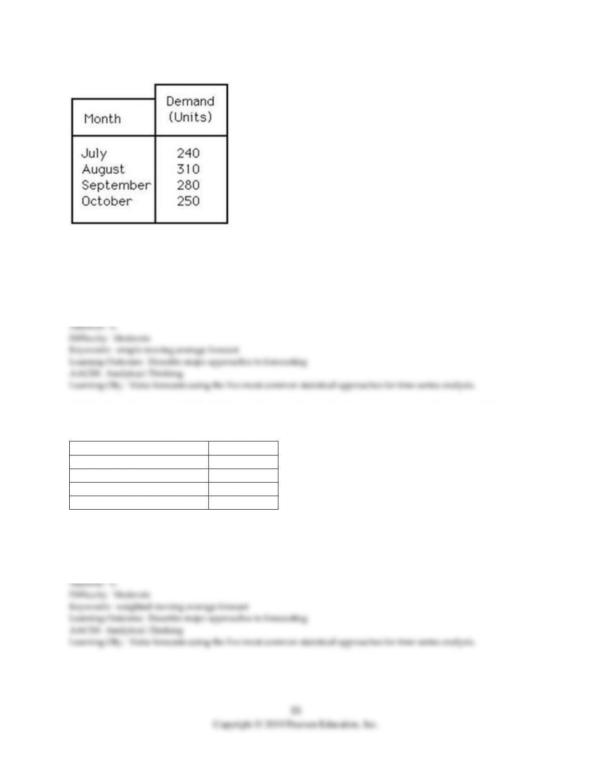
Table 8.5
14) Use the information in Table 8.5. Using the simple moving-average technique for the most recent
three months, what will be the forecasted demand for November?
A) fewer than or equal to 260 units
B) greater than 260, but fewer than or equal to 275 units
C) greater than 275, but fewer than or equal to 290 units
D) more than 290 units
15) Use the information in Table 8.5. Using the 4-month weighted moving-average technique and the
following weights, what is the forecasted demand for November?
Time Period
Weight
Most recent month
50%
One month ago
20%
Two months ago
20%
Three months ago
10%
A) fewer than or equal to 250 units
B) greater than 250 but fewer than or equal to 265 units
C) greater than 265 but fewer than or equal to 280 units
D) more than 280 units
16) Use the information in Table 8.5. Using the exponential smoothing method, with alpha equal to 0.2,
what is the forecasted demand for November? Use an initial value for the forecast equal to 277 units.
A) fewer than or equal to 260 units
B) greater than 260 but fewer than or equal to 275 units
C) greater than 275 but fewer than or equal to 285 units
D) more than 285 units
17) Use the information in Table 8.6. Use an exponential smoothing model with a smoothing parameter of
0.30 and an April forecast of 525 to determine what the forecast sales would have been for June.
A) fewer than or equal to 535
B) greater than 535 but fewer than or equal to 545
C) greater than 545 but fewer than or equal to 555
D) greater than 555
18) Use the information in Table 8.6. Use the exponential smoothing method with = 0.5 and a February
forecast of 500 to forecast the sales for May.
A) fewer than or equal to 530
B) greater than 530 but fewer than or equal to 540
C) greater than 540 but fewer than or equal to 550
D) greater than 550

Table 8.7
A sales manager wants to forecast monthly sales of the machines the company makes using the following
monthly sales data.
Month
Balance
1
$3,803
2
$2,558
3
$3,469
4
$3,442
5
$2,682
6
$3,469
7
$4,442
8
$3,728
19) Use the information in Table 8.7. Forecast the monthly sales of the machine for month 9, using the
three-month moving-average method.
A) $3,728
B) $4,085
C) $3,880
D) $3,277
20) Use the information in Table 8.7. Use the 3-month weighted moving-average method to calculate the
forecast for month 9. The weights are 0.60, 0.30, and 0.10, where 0.60 refers to the most recent demand.
A) $3,916
B) $3,880
C) $3,396
D) $3,229

21) Use the information in Table 8.7. If the forecast for period 7 is $4,300, what is the forecast for period 9
using exponential smoothing with an alpha equal to 0.30?
A) $4,300
B) $4,342
C) $4,158
D) $3,957
22) Use the information in Table 8.7. What is the forecast for period 9 using a naive forecast?
A) $3,728
B) $3,803
C) $4,442
D) $4,085
23) Which statement about forecast accuracy is true?
A) A manager must be careful not to “overfit” past data.
B) The ultimate test of forecasting power is how well a model fits past data.
C) The ultimate test of forecasting power is how a model fits holdout samples.
D) The best technique in explaining past data is the best technique to predict the future.
24) A forecaster that uses a holdout set approach as a final test for forecast accuracy typically uses:
A) the entire data set available to develop the forecast.
B) the older observations in the data set to develop the forecast and more recent to check accuracy.
C) the newer observations in the data set to develop the forecast and older observations to check
accuracy.
D) every other observation to develop the forecast and the remaining observations to check the accuracy.