
37) What is the trend component of Holt’s model for period 0?
A) -2.5
B) 10.3
C) 2.5
D) 6.4
38) What is the level component of Holt’s model for period 0?
A) -2.5
B) 10.3
C) 2.5
D) 6.4
Scenario 7.2 — Gulab Greatness
Historical demand for gulab jamun from a sweet stall on Commercial Road is as displayed in the
table.
Month
Demand
(orders)
January
66,753
February
67,686
March
68,641
April
68,979
May
69,278
June
69,577
July
69,602
August
70,348
September
70,806
October
71,011
November
71,819
December
72,752
39) Use a simple moving average of three periods to forecast the demand for October. What is
the forecast?
A) 70,252
B) 70,722
C) 69,842
D) 71,212
40) Use exponential smoothing to forecast the demand for July. What is the forecast if α = 0.4
and the forecast for May was 69,000?
A) 69,346
B) 69,379
C) 69,500
D) 69,298
41) What is the trend component of Holt’s model for period 0?
A) 642
B) 66,768
C) 462
D) 78,666
42) What is the level component of Holt’s model for period 0?
A) 78,666
B) 642
C) 462
D) 66,768
43) What is the forecast for June using Holt’s model with an alpha of 0.1 and a beta of 0.2?
A) 69,612
B) 69,121
C) 70,082
D) 70,499
44) The measure of forecast error where the amount of error of each forecast is squared and then
an average is calculated is
A) mean squared error (MSE).
B) mean absolute deviation (MAD).
C) mean absolute percentage error (MAPE).
D) the tracking signal.
45) The measure of forecast error where the absolute amount of error of each forecast is
averaged is
A) mean squared error (MSE).
B) mean absolute deviation (MAD).
C) mean absolute percentage error (MAPE).
D) bias.
46) The measure of forecast error where the average absolute error of each forecast is shown as a
percentage of demand is
A) mean squared error (MSE).
B) mean absolute percentage error (MAPE).
C) bias.
D) the tracking signal.
47) The measure of whether a forecast method consistently over- or underestimates demand is
A) mean absolute deviation (MAD).
B) mean absolute percentage error (MAPE).
C) bias.
D) the tracking signal.
48) The measure of how significantly a forecast method consistently over- or underestimates
demand is
A) mean squared error (MSE).
B) mean absolute deviation (MAD).
C) bias.
D) the tracking signal.

20
49) Which of the following is a commonly used measure for measuring forecast error?
A) MDE
B) MKE
C) MAD
D) MES
50) The ________ is a good measure of forecast error when the underlying forecast has
significant seasonality and demand varies considerably from one period to the next.
A) MAD
B) MSE
C) MKE
D) MAPE
Scenario 7.3
The Entrepreneurship professor had a habit of oversupplying extra credit opportunities for his
class each semester and his colleagues delighted in trying to forecast his class enrollment from
one semester to the next. The forecasts for one colleague, along with the actual class enrollment,
appear in the table.
Period
Actual
Forecast
1
173
166.7
2
177
183
3
180
174.7
4
151
163.2
5
168
155.6
6
184
187.6
7
198
192.9
8
191
194.6
9
167
149.8
10
177
195.2
51) Calculate the MAD for this scenario.
A) 10.04
B) 8.99
C) 10.40
D) 9.25
52) Calculate the MSE for this scenario.
A) 106.60
B) 119.80
C) 108.54
D) 112.20
53) What is the largest value for the tracking signal (either under or overforecasting)?
A) 0.955
B) -3.188
C) 1.004
D) 2.623
54) What is the mean absolute percentage error?
A) 5.24%
B) 5.61%
C) 5.40%
D) 5.06%
55) Use Solver to determine the alpha that minimizes the MAD for the exponential smoothing
forecast for the data that appear in this table. Use the actual demand of period 1 as the forecast
for period 2 and then use the forecasts for periods 2 through 9 to calculate MAD.
Period
Demand
1
272
2
278
3
269
4
280
5
267
6
258
7
278
8
298
9
286
10
290
A) 0.36
B) 0.43
C) 0.54
D) 0.62
56) Use Solver to determine the alpha that minimizes the MSE for the exponential smoothing
forecast for the data that appear in this table. Use the actual demand of period 1 as the forecast
for period 2 and then use the forecasts for periods 2 through 9 to calculate MSE.
Period
Demand
1
272
2
278
3
269
4
280
5
267
6
258
7
278
8
298
9
286
10
290
A) 0.39
B) 0.48
C) 0.57
D) 0.66
57) What Excel function/feature should be used to calculate a moving average?
A) Solver
B) =AVERAGE
C) =MAVE
D) Goal seek
58) What Excel function/feature should be used to minimize the mean squared error for an
exponential smoothing model?
A) Solver
B) =EXPON
C) =ALPHA
D) Goal seek
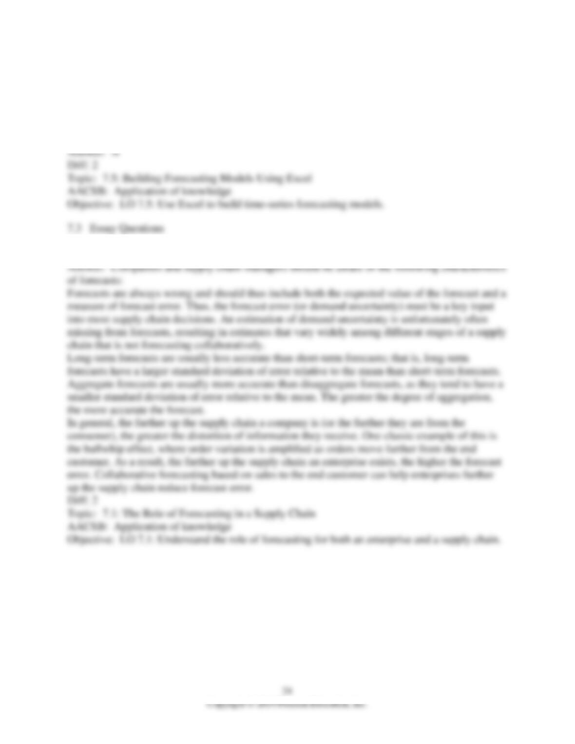
1) Describe the basic characteristics of forecasts that managers should be aware of.

25
2) Explain the basic, six-step approach to help an organization perform effective forecasting.
Answer: The following basic, six-step approach helps an organization perform effective
forecasting:

26
Scenario 7.4 – Marshmallow Madness
Historical demand for Peeps is as displayed in the table.
Month
Demand
January
11
February
18
March
31
April
39
May
44
June
53
July
67
August
82
September
96
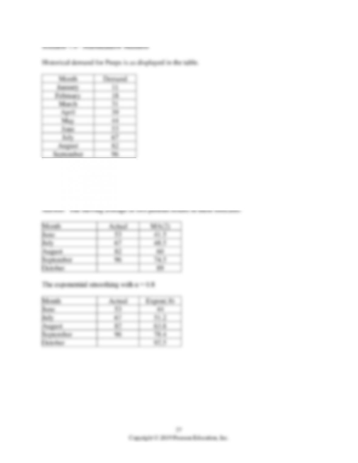
3) Develop forecasts for June through October using these techniques: moving average of two
period, simple exponential smoothing with an alpha of 0.8, and Holt’s method. For the
exponential smoothing model assume that the forecast for May is the actual demand for May.
Comment on the use of these three methods to generate a forecast in this situation.
53
67
82
60
96
89
53
44
67
82
96
28
Copyright © 2019 Pearson Education, Inc.
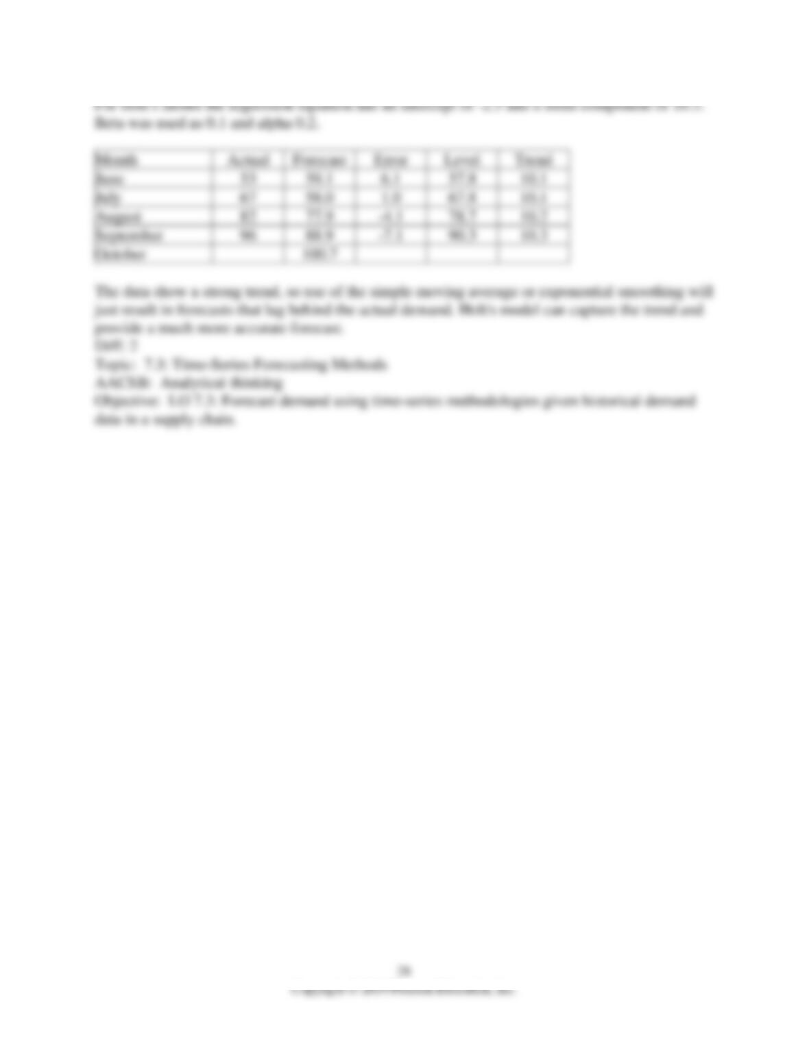
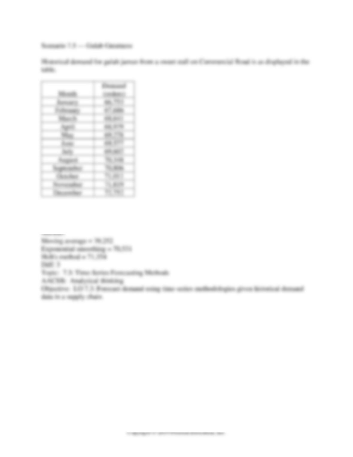
For Holt’s model the regression equation has an intercept of -2.5 and a trend component of 10.3.
Beta was used as 0.1 and alpha 0.2.
Month
Actual
Forecast
Error
Level
Trend
June
53
59.1
6.1
57.8
10.1
July
67
58.0
1.0
67.8
10.1
August
82
77.9
-4.1
78.7
10.2
September
96
88.9
-7.1
90.3
10.3
October
100.7
The data show a strong trend, so use of the simple moving average or exponential smoothing will
just result in forecasts that lag behind the actual demand. Holt’s model can capture the trend and
provide a much more accurate forecast.
Diff: 2
Topic: 7.3: Time-Series Forecasting Methods
AACSB: Analytical thinking
Objective: LO 7.3: Forecast demand using time-series methodologies given historical demand
data in a supply chain.
29
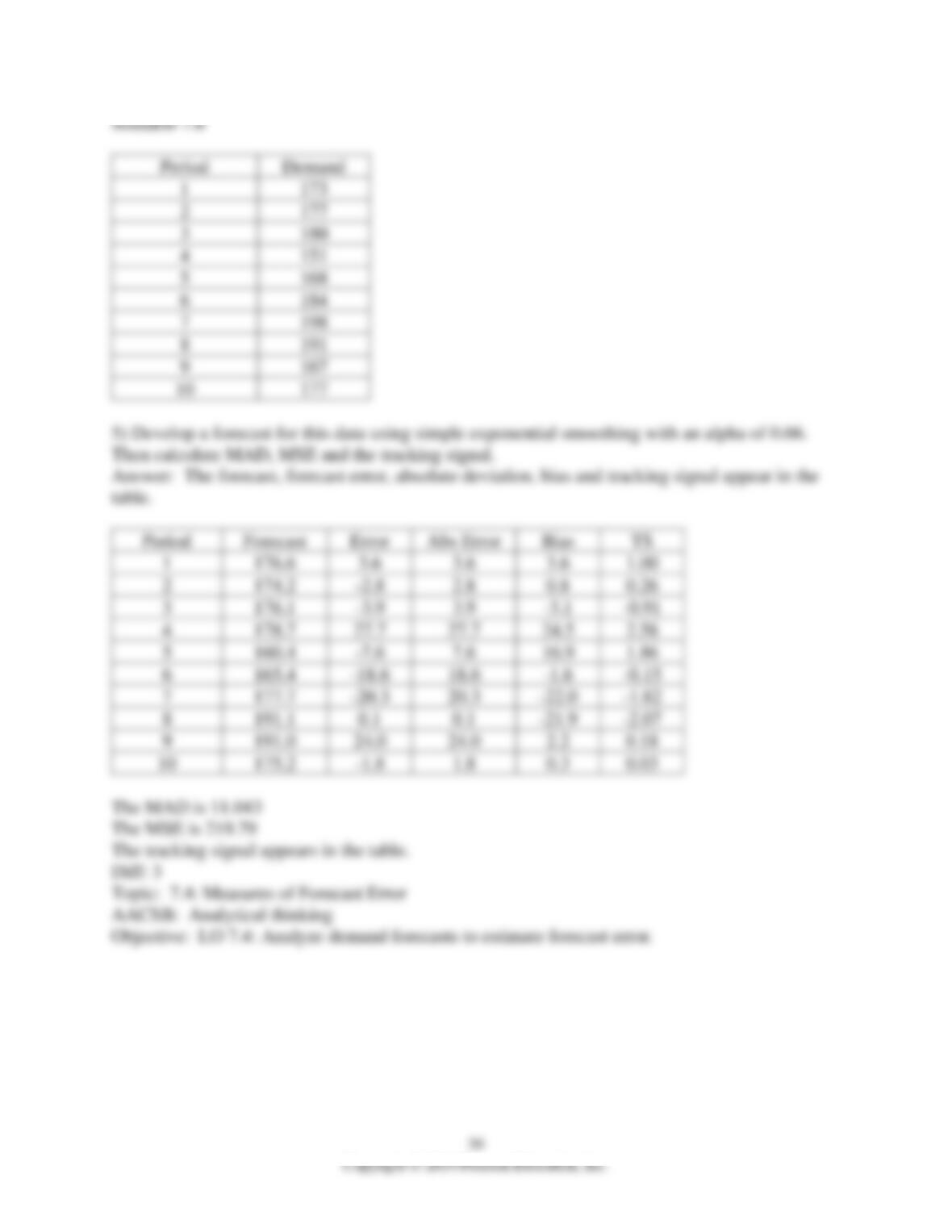
Scenario 7.5 — Gulab Greatness
Historical demand for gulab jamun from a sweet stall on Commercial Road is as displayed in the
table.
Month
Demand
(orders)
January
66,753
February
67,686
March
68,641
April
68,979
May
69,278
June
69,577
July
69,602
August
70,348
September
70,806
October
71,011
November
71,819
December
72,752
4) Use a simple moving average of three periods to forecast the demand for October. Then use
exponential smoothing with an alpha = 0.4 to forecast October, assuming an August forecast
equal to August demand. Finally, use Holt’s method with an alpha of 0.2 and a beta of 0.3.
30
Copyright © 2019 Pearson Education, Inc.
Scenario 7.6
Period
Demand
1
173
2
177
3
180
4
151
5
168
6
184
7
198
8
191
9
167
10
177
5) Develop a forecast for this data using simple exponential smoothing with an alpha of 0.66.
Then calculate MAD, MSE and the tracking signal.
Answer: The forecast, forecast error, absolute deviation, bias and tracking signal appear in the
table.
Period
Forecast
Error
Abs Error
Bias
TS
1
176.6
3.6
3.6
3.6
1.00
2
174.2
-2.8
2.8
0.8
0.26
3
176.1
-3.9
3.9
-3.1
-0.91
4
178.7
27.7
27.7
24.5
2.58
5
160.4
-7.6
7.6
16.9
1.86
6
165.4
-18.6
18.6
-1.6
-0.15
7
177.7
-20.3
20.3
-22.0
-1.82
8
191.1
0.1
0.1
-21.9
-2.07
9
191.0
24.0
24.0
2.2
0.18
10
175.2
-1.8
1.8
0.3
0.03
The MAD is 11.043
The MSE is 219.79
The tracking signal appears in the table.
Diff: 3
Topic: 7.4: Measures of Forecast Error
AACSB: Analytical thinking
Objective: LO 7.4: Analyze demand forecasts to estimate forecast error.