1. The enduring increment in the common price value of services and products in
an economy over a range of time is normally known as inflation. As the normal cost
value ascents, all currency has the tendency to purchase fewer products and services;
along these lines, a decrease in the ability to buy per unit of cash is drawn in inflation
which is a loss of the actual price in the mechanism of trade and unit of account inside
the household management. The ability to purchase of every unit of currency is
diminishing because inflation creates the cost of products and services to face an
increment after some time. Consequently, it increases the cost of living.
To gauge the value of the cost of products and services facing an increment or
abatement, we use the inflation rate. It is the rate increment or reduction in costs
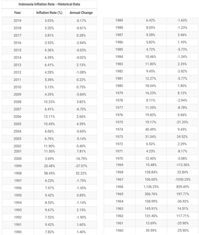
throughout an indicated time frame, normally yearly. Below are the Inflation rate data
of Indonesia for 59 years from 1960 until 2019 along with its annual change.

Measuring the yearly inflation rate of the economy of a country and comparing one
year to another have a lot of functions for the economic growth of a country. For example, it
can help economists and policymakers to create a proper policy to encounter certain condition.
It can also be used to predict future annual rate. For instance, Bank Indonesia predicted that in
2020, the Inflation rate of Indonesia will reach 3.10% or 0.07% higher than in 2019 from the
data provided.
In this report, using a statistical method, hypothesis testing and with 95% confidence
interval, we want to determine whether the annual change of inflation rate of Indonesia from
2019 – 2020 is or differs from 0.07%. Or In other words, is the claim that Indonesia’s inflation
rate in 2020 will increase by 0.07% reasonable. To conduct the hypothesis testing, we first take
20 random samples from the data to measure future annual rate. Below are 20 samples taken
from Indonesia inflation rate annual change data :
Year
Inflation rate
Annual change
1961
13.69%
-25.90%
1964
108.99%
-36.92%
1969
15.48%
-113.36%
1974
40.49%
9.45%
1977
11.05%
-8.78%
1979
16.23%
8.12%
1982
9.45%
-2.82%
1986
5.82%
1.10%
1989
6.42%
-1.63%
1992
7.52%
-1.90%
1994
8.53%
-1.14%
1997
6.23%
-1.75%
1999
20.48%
-37.97%
2004
6.06%
-0.69%
2006
13.11%
2.66%
2009
4.39%
-5.84%
2012
4.28%
-1.08%
From the samples depicted above, we know that the sample size(n) is 20. We also need
to calculate the measure of location (i.e. mean, median, and mode) and the measure of
dispersion (range, standard deviation, and variance) to calculate the confidence interval
estimates and the value of tdf.
Sample Mean (X) = -11.07%
Sample median = -1.69%
Sample mode = 9.45%
Sample range = 122.81%
Sample Standard deviation (S) = 0.273153829 (27.3%)
Sample Variance = 0.074613014 (7.46%)
Since the population standard deviation (𝜎) is unknown, we use t distribution to find
the value of confidence interval estimates and hypothesis testing. The formula for confidence
interval with unknown 𝜎 is :
C.I. = X ± t 𝑠
√𝑛
The value of t = tdf = 2.093 (from t distribution table)
With df = n-1 = 20-1 = 19 and 𝛼 = 0.05
Therefore, Confidence Interval :
C.I. = -11.07% ± 2.0930.273153829
√20 = -11.07% ± 0.014292774
C.I. = (-0.096407226, 0.096407226) or (-9.64%,9.64%)
2014
6.39%
-0.02%
2016
3.53%
-2.84%
2019
3.03%
-0.17%
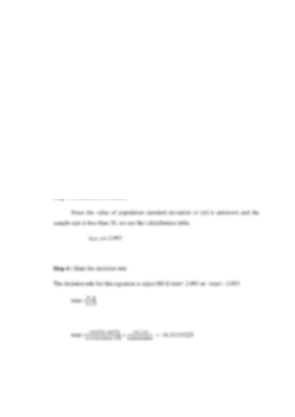
From the calculation of confidence interval estimates, the interval value is between 9.64 %
and -9.64%
After calculating the confidence interval estimates, we then can proceed to conduct
the hypothesis testing.
Step 1 : State the null hypothesis and the alternate hypothesis
H0 :𝜇 = 0.07%
H1 :𝜇 ≠ 0.07%
Step 2 : Select the level of significance
𝛼 = 0.05