Why This Chapter Matters to You
In your
professional
life
ACCOUNTING You need to understand how to calculate and analyze
operating and financial leverage and to be familiar with the tax and
earnings effects of various capital structures.
INFORMATION SYSTEMS You need to understand the types of capital
and what capital structure is because you will provide much of the
information needed in management’s determination of the best capital
structure for the firm.
MANAGEMENT You need to understand leverage so that you can con-
trol risk and magnify returns for the firm’s owners and to understand
capital structure theory so that you can make decisions about the firm’s
optimal capital structure.
MARKETING You need to understand breakeven analysis, which you
will use in pricing and product feasibility decisions.
OPERATIONS You need to understand the impact of fixed and variable
operating costs on the firm’s breakeven point and its operating
leverage because these costs will have a major impact on the firm’s risk
and return.
Like corporations, you routinely
incur debt, using both credit cards
for short-term needs and negotiated long-term loans. When you borrow
over the long term, you experience the benefits and consequences of
leverage. Also, the level of your outstanding debt relative to net worth
is conceptually the same as a firm’s capital structure. It reflects your
financial risk and affects the availability and cost of borrowing.
In your
personal
life
Learning Goals
Discuss leverage, capital
structure, breakeven analysis, the
operating breakeven point, and
the effect of changing costs on the
breakeven point.
Understand operating, financial,
and total leverage and the
relationships among them.
Describe the types of capital,
external assessment of capital
structure, the capital structure of
non–U.S. firms, and capital
structure theory.
Explain the optimal capital
structure using a graphical view
of the firm’s cost-of-capital
functions and a zero-growth
valuation model.
Discuss the EBIT–EPS approach to
capital structure.
Review the return and risk of
alternative capital structures, their
linkage to market value, and
other important considerations
related to capital structure.
LG 6
LG 5
LG 4
LG 3
LG 2
LG 1
13 Leverage and Capital
Structure
506

507
Trading Equity for Debt
As the broader U.S. stock market roared back to
life in 2009, shares in the biotechnology firm,
Genzyme, dropped 28 percent. Contamination prob-
lems at Genzyme’s main manufacturing facility
prompted the firm to stop production during the
cleanup, and that in turn led to production shortages of
some of the firms best-selling drugs. That performance
irked one of Genzyme’s largest shareholders, Carl
Icahn, who promptly launched a proxy fight to gain four seats on the company’s board of direc-
tors. In June 2010, Genzyme reached an agreement with Icahn giving his representatives two
seats on their board.
Just eight days later, Genzyme’s stock rose 3.7 percent on the announcement that the com-
pany would issue $1 billion in debt. Genzyme planned to use the proceeds from the issue,
along with $1 billion in cash reserves, to repurchase approximately 40 million shares of
common stock. That move represented a significant shift in the firm’s capital structure (that is, its
mix of debt and equity financing), a move that would put more cash in the hands of share-
holders and apply more pressure on Genzyme management to generate positive cash flow from
the business. With more of its financing coming from debt, Genzyme was adding financial
leverage to its business, meaning that if the firm succeeds in selling its products, the returns to
shareholders will be magnified. However, if Genzyme instead experiences further declines in its
business, paying back the debt may prove to be difficult, and returns to shareholders will suffer
as a result.
Genzyme Corp.

508 PART 6 Long-Term Financial Decisions
13.1 Leverage
Leverage refers to the effects that fixed costs have on the returns that shareholders
earn. By “fixed costs” we mean costs that do not rise and fall with changes in a
firm’s sales. Firms have to pay these fixed costs whether business conditions are
good or bad. These fixed costs may be operating costs, such as the costs incurred
by purchasing and operating plant and equipment, or they may be financial costs,
such as the fixed costs of making debt payments. Generally, leverage magnifies
both returns and risks. A firm with more leverage may earn higher returns on
average than a firm with less leverage, but the returns on the more leveraged firm
will also be more volatile.
Many business risks are out of the control of managers, but not the risks
associated with leverage. Managers can limit the impact of leverage by adopting
strategies that rely more heavily on variable costs than on fixed costs. For
example, a basic choice that many firms confront is whether to make their own
products or to outsource manufacturing to another firm. A company that does its
own manufacturing may invest billions in factories around the world. These fac-
tories generate costs whether they are running or not. In contrast, a company that
outsources production can completely eliminate its manufacturing costs simply
by not placing orders. Costs for a firm like this are more variable and will gener-
ally rise and fall as demand warrants.
In the same way, managers can influence leverage in their decisions about
how the company raises money to operate. The amount of leverage in the firm’s
capital structure—the mix of long-term debt and equity maintained by the firm—
can significantly affect its value by affecting return and risk. The more debt a firm
issues, the higher are its debt repayment costs, and those costs must be paid
regardless of how the firm’s products are selling. Because leverage can have such
a large impact on a firm, the financial manager must understand how to measure
and evaluate leverage, particularly when making capital structure decisions.
Table 13.1 uses an income statement to highlight where different sources of
leverage come from.
LG 1
leverage
Refers to the effects that fixed
costs have on the returns that
shareholders earn; higher
leverage generally results in
higher but more volatile
returns.
capital structure
The mix of long-term debt and
equity maintained by the firm.
General Income Statement Format and Types of Leverage
Sales revenue
Less: Cost of goods sold
Operating leverage Gross profits
Less: Operating expenses
Earnings before interest and taxes (EBIT)
Less: Interest Total leverage
Net profits before taxes
Less: Taxes
Financial leverage Net profits after taxes
Less: Preferred stock dividends
Earnings available for common stockholders
Earnings per share (EPS)
TABLE 13.1
LG 2

•Operating leverage is concerned with the relationship between the firm’s sales
revenue and its earnings before interest and taxes (EBIT) or operating profits.
When costs of operations (such as cost of goods sold and operating expenses) are
largely fixed, small changes in revenue will lead to much larger changes in EBIT.
•Financial leverage is concerned with the relationship between the firm’s EBIT
and its common stock earnings per share (EPS). On the income statement, you
can see that the deductions taken from EBIT to get to EPS include interest,
taxes, and preferred dividends. Taxes are clearly variable, rising and falling
with the firm’s profits, but interest expense and preferred dividends are usu-
ally fixed. When these fixed items are large (that is, when the firm has a lot of
financial leverage), small changes in EBIT produce larger changes in EPS.
•Total leverage is the combined effect of operating and financial leverage. It is
concerned with the relationship between the firm’s sales revenue and EPS.
We will examine the three types of leverage concepts in detail. First, though,
we will look at breakeven analysis, which lays the foundation for leverage con-
cepts by demonstrating the effects of fixed costs on the firm’s operations.
BREAKEVEN ANALYSIS
Firms use breakeven analysis, also called cost-volume-profit analysis, (1) to deter-
mine the level of operations necessary to cover all costs and (2) to evaluate the
profitability associated with various levels of sales. The firm’s operating
breakeven point is the level of sales necessary to cover all operating costs. At that
point, earnings before interest and taxes (EBIT) equals $0.1
The first step in finding the operating breakeven point is to divide the cost of
goods sold and operating expenses into fixed and variable operating costs. Fixed
costs are costs that the firm must pay in a given period regardless of the sales
volume achieved during that period. These costs are typically contractual; rent,
for example, is a fixed cost. Because fixed costs do not vary with sales, we typi-
cally measure them relative to time. For example, we would typically measure
rent as the amount due per month. Variable costs vary directly with sales volume.
Shipping costs, for example, are a variable cost.2We typically measure variable
costs in dollars per unit sold.
Algebraic Approach
Using the following variables, we can recast the operating portion of the firm’s
income statement given in Table 13.1 into the algebraic representation shown in
Table 13.2.
VC =variable operating cost per unit
FC =fixed operating cost per period
Q=sales quantity in units
P=sale price per unit
CHAPTER 13 Leverage and Capital Structure 509
1. Quite often, the breakeven point is calculated so that it represents the point at which all costs—both operating
and financial—are covered. For now, we focus on the operating breakeven point as a way to introduce the concept
of operating leverage. We will discuss financial leverage later.
2. Some costs, commonly called semifixed or semivariable, are partly fixed and partly variable. An example is sales
commissions that are fixed for a certain volume of sales and then increase to higher levels for higher volumes. For
convenience and clarity, we assume that all costs can be classified as either fixed or variable.
breakeven analysis
Used to indicate the level of
operations necessary to cover
all costs and to evaluate the
profitability associated with
various levels of sales; also
called
cost-volume-profit
analysis
.
operating breakeven point
The level of sales necessary to
cover all
operating costs;
the
point at which EBIT $0.=

Rewriting the algebraic calculations in Table 13.2 as a formula for earnings
before interest and taxes yields Equation 13.1:
(13.1)
Simplifying Equation 13.1 yields:
(13.2)
As noted above, the operating breakeven point is the level of sales at which all
fixed and variable operating costs are covered—the level at which EBIT equals
$0. Setting EBIT equal to $0 and solving Equation 13.2 for Qyields:
(13.3)
Qis the firm’s operating breakeven point.3
Assume that Cheryl’s Posters, a small poster retailer, has fixed operating costs of
$2,500. Its sale price is $10 per poster, and its variable operating cost is $5 per
poster. Applying Equation 13.3 to these data yields:
At sales of 500 units, the firm’s EBIT should just equal $0. The firm will have
positive EBIT for sales greater than 500 units and negative EBIT, or a loss, for
sales less than 500 units. We can confirm this by substituting values above and
below 500 units, along with the other values given, into Equation 13.1.
Q=$2,500
$10 –$5 =$2,500
$5 =500 units
Example 13.1 3
Q=FC
P–VC
EBIT =Q*(P–VC)–FC
EBIT =(P*Q)–FC –(VC *Q)
510 PART 6 Long-Term Financial Decisions
Operating Leverage, Costs, and Breakeven Analysis
Algebraic
Item representation
Sales revenue (PQ)
Operating leverage Less: Fixed operating costs FC
Less: Variable operating costs
Earnings before interest and taxes EBIT
–(VC *Q)
–
*
TABLE 13.2
3. Because the firm is assumed to be a single-product firm, its operating breakeven point is found in terms of unit
sales, Q. For multiproduct firms, the operating breakeven point is generally found in terms of dollar sales, S. This is
done by substituting the contribution margin, which is 100 percent minus total variable operating costs as a per-
centage of total sales, denoted VC%, into the denominator of Equation 13.3. The result is Equation 13.3a:
(13.3a)
This multiproduct-firm breakeven point assumes that the firm’s product mix remains the same at all levels of sales.
S=FC
1–VC%
Graphical Approach
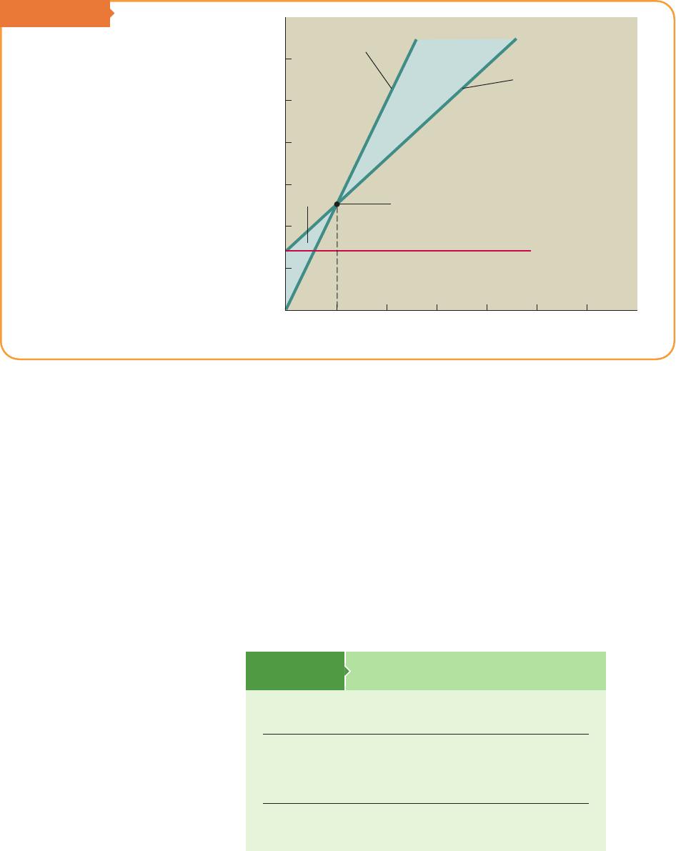
Figure 13.1 presents in graphical form the breakeven analysis of the data in the
preceding example. The firm’s operating breakeven point is the point at which its
total operating cost—the sum of its fixed and variable operating costs—equals
sales revenue. At this point, EBIT equals $0. The figure shows that for sales
below 500 units, total operating cost exceeds sales revenue, and EBIT is less than
$0 (a loss). For sales above the breakeven point of 500 units, sales revenue
exceeds total operating cost, and EBIT is greater than $0.
Changing Costs and the Operating Breakeven Point
A firm’s operating breakeven point is sensitive to a number of variables: fixed
operating cost (FC), the sale price per unit (P), and the variable operating cost per
unit (VC). Refer to Equation 13.3 to see how increases or decreases in these vari-
ables affect the breakeven point. The sensitivity of the breakeven sales volume
(Q) to an increase in each of these variables is summarized in Table 13.3. As
CHAPTER 13 Leverage and Capital Structure 511
Sales
Revenue
Total
Operating
Cost
Operating
Breakeven
Point
EBIT
Fixed
Operating
Cost
5000 1,000 1,500 2,000 2,500 3,000
Loss
12,000
10,000
8,000
6,000
4,000
2,000
Costs/Revenues ($)
Sales (units)
FIGURE 13.1
Breakeven Analysis
Graphical operating
breakeven analysis
Sensitivity of Operating Breakeven Point
to Increases in Key Breakeven Variables
Effect on operating
Increase in variable breakeven point
Fixed operating cost (FC) Increase
Sale price per unit (P) Decrease
Variable operating cost per unit (VC) Increase
Note: Decreases in each of the variables shown would have the opposite
effect on the operating breakeven point.
TABLE 13.3
might be expected, an increase in cost (FC or VC) tends to increase the operating
breakeven point, whereas an increase in the sale price per unit (P) decreases the
operating breakeven point.
Assume that Cheryl’s Posters wishes to evaluate the impact of several options:
(1) increasing fixed operating costs to $3,000, (2) increasing the sale price per
unit to $12.50, (3) increasing the variable operating cost per unit to $7.50, and
(4) simultaneously implementing all three of these changes. Substituting the
appropriate data into Equation 13.3 yields the following results:
Comparing the resulting operating breakeven points to the initial value of 500
units, we can see that the cost increases (actions 1 and 3) raise the breakeven
point, whereas the revenue increase (action 2) lowers the breakeven point. The
combined effect of increasing all three variables (action 4) also results in an
increased operating breakeven point.
Rick Polo is considering having a new fuel-saving device
installed in his car. The installed cost of the device is $240 paid
up front, plus a monthly fee of $15. He can terminate use of the device any time
without penalty. Rick estimates that the device will reduce his average monthly
gas consumption by 20%, which, assuming no change in his monthly mileage,
translates into a savings of about $28 per month. He is planning to keep the car
for 2 more years and wishes to determine whether he should have the device
installed in his car.
To assess the financial feasibility of purchasing the device, Rick calculates
the number of months it will take for him to break even. Letting the installed
cost of $240 represent the fixed cost (FC), the monthly savings of $28 repre-
sent the benefit (P), and the monthly fee of $15 represent the variable cost
(VC), and substituting these values into the breakeven point equation,
Equation 13.3, we get:
Because the fuel-saving device pays itself back in 18.5 months, which is less than
the 24 months that Rick is planning to continue owning the car, he should have
the fuel-saving device installed in his car.
=18.5 months
Breakeven point (in months) =$240 ,($28 –$15) =$240 ,$13
Personal Finance Example 13.3 3
(4) Operating breakeven point =$3,000
$12.50 –$7.50 =600 units
(3) Operating breakeven point =$2,500
$10 –$7.50 =1,000 units
(2) Operating breakeven point =$2,500
$12.50 –$5 =3331
>3 units
(1) Operating breakeven point =$3,000
$10 –$5 =600 units
Example 13.2 3
512 PART 6 Long-Term Financial Decisions
OPERATING LEVERAGE
Operating leverage results from the existence of fixed costs that the firm must pay
to operate. Using the structure presented in Table 13.2, we can define operating
leverage as the use of fixed operating costs to magnify the effects of changes in
sales on the firm’s earnings before interest and taxes.
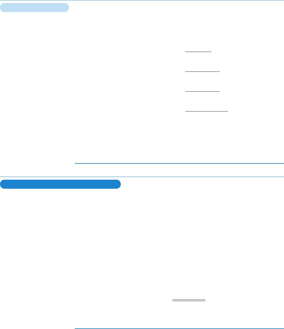
Using the data for Cheryl’s Posters (sale price, P$10 per unit; variable oper-
ating cost, VC $5 per unit; fixed operating cost, FC $2,500), Figure 13.2
presents the operating breakeven graph originally shown in Figure 13.1. The
additional notations on the graph indicate that as the firm’s sales increase from
1,000 to 1,500 units (Q1to Q2), its EBIT increases from $2,500 to $5,000 (EBIT1
to EBIT2). In other words, a 50% increase in sales (1,000 to 1,500 units) results
in a 100% increase in EBIT ($2,500 to $5,000). Table 13.4 includes the data for
Figure 13.2 as well as relevant data for a 500-unit sales level. We can illustrate
two cases using the 1,000-unit sales level as a reference point.
Case 1 A 50% increase in sales (from 1,000 to 1,500 units) results in a 100%
increase in earnings before interest and taxes (from $2,500 to $5,000).
Case 2 A 50% decrease in sales (from 1,000 to 500 units) results in a 100%
decrease in earnings before interest and taxes (from $2,500 to $0).
From the preceding example, we see that operating leverage works in both
directions. When a firm has fixed operating costs, operating leverage is present.
== =
Example 13.4 3
CHAPTER 13 Leverage and Capital Structure 513
operating leverage
The use of
fixed operating
costs
to magnify the effects of
changes in sales on the firm’s
earnings before interest and
taxes.
2,000
4,000
6,000
8,000
10,000
12,000
14,000
16,000
5000 1,000 1,500 2,000 2,500 3,000
Q1Q2
Sales (units)
Costs/Revenues ($)
EBIT1
$2,500
EBIT2
$5,000
Loss
EBIT
Fixed
Operating
Cost
Total
Operating
Cost
Sales
Revenue
FIGURE 13.2
Operating Leverage
Breakeven analysis and
operating leverage

An increase in sales results in a more-than-proportional increase in EBIT; a
decrease in sales results in a more-than-proportional decrease in EBIT.
Measuring the Degree of Operating Leverage (DOL)
The degree of operating leverage (DOL) is a numerical measure of the firm’s
operating leverage. It can be derived using the following equation:4
(13.4)
Whenever the percentage change in EBIT resulting from a given percentage
change in sales is greater than the percentage change in sales, operating leverage
exists. This means that as long as DOL is greater than 1, there is operating
leverage.
Applying Equation 13.4 to cases 1 and 2 in Table 13.4 yields the following results:
Case 1:
Case 2:
Because the result is greater than 1, operating leverage exists. For a given base
level of sales, the higher the value resulting from applying Equation 13.4, the
greater the degree of operating leverage.
–100%
–50% =2.0
+100%
+50% =2.0
Example 13.5 3
DOL =Percentage change in EBIT
Percentage change in sales
514 PART 6 Long-Term Financial Decisions
TABLE 13.4
4. The degree of operating leverage also depends on the base level of sales used as a point of reference. The closer the
base sales level used is to the operating breakeven point, the greater the operating leverage. Comparison of the
degree of operating leverage of two firms is valid only when the same base level of sales is used for both firms.
degree of operating
leverage (DOL)
The numerical measure of the
firm’s operating leverage.
The EBIT for Various Sales Levels
Case 2 Case 1
⫺50% ⫹50%
Sales (in units) 500 1,000 1,500
Sales revenuea$5,000 $10,000 $15,000
Less: Variable operating costsb2,500 5,000 7,500
Less: Fixed operating costs
Earnings before interest and taxes (EBIT) $ 0 $ 2,500 $ 5,000
⫺100% ⫹100%
aSales revenue $10/unit sales in units.
bVariable operating costs $5/unit sales in units.*=
*=
2,5002,5002,500
A more direct formula for calculating the degree of operating leverage at a
base sales level, Q, is shown in Equation 13.5.5
(13.5)
Substituting , and into Equation
13.5 yields the following result:
The use of the formula results in the same value for DOL (2.0) as that found by
using Table 13.4 and Equation 13.4.6
See the Focus on Practice box for a discussion of operating leverage at software
maker Adobe.
DOL at 1,000 units =1,000 *($10 –$5)
1,000 *($10 –$5) –$2,500 =$5,000
$2,500 =2.0
FC =$2,500Q=1,000, P=$10, VC =$5
Example 13.6 3
DOL at base sales level Q =Q*(P–VC)
Q*(P–VC)–FC
CHAPTER 13 Leverage and Capital Structure 515
5. Technically, the formula for DOL given in Equation 13.5 should include absolute value signs because it is possible
to get a negative DOL when the EBIT for the base sales level is negative. Because we assume that the EBIT for the
base level of sales is positive, we do not use the absolute value signs.
6. When total revenue in dollars from sales—instead of unit sales—is available, the following equation, in which
TR total revenue in dollars at a base level of sales and TVC total variable operating costs in dollars, can be used:
This formula is especially useful for finding the DOL for multiproduct firms. It should be clear that because in the
case of a single-product firm, , substitution of these values into Equation 13.5
results in the equation given here.
TR =Q*P and TVC =Q*VC
DOL at base dollar sales TR =TR –TVC
TR –TVC –FC
==
focus on PRACTICE
Adobe’s Leverage
2009. A 22.6 percent increase in
2007 sales resulted in EBIT growth of
39.7 percent. In 2008, EBIT increased
just a little faster than sales did, but in
2009 as the economy endured a severe
recession, Adobe revenues plunged
17.7 percent. The effect of operating
leverage was that EBIT declined even
faster, posting a 35.3 percent drop.
3
Summarize the pros and cons of
operating leverage.
development and initial marketing stages.
The up-front development costs are fixed,
and subsequent production costs are
practically zero. The economies of scale
are huge: Once a company sells enough
copies to cover its fixed costs, incremen-
tal dollars go primarily to profit.
As demonstrated in the following
table, operating leverage magnified
Adobe’s
increase
in EBIT in 2007 while
magnifying the
decrease
in EBIT in
Adobe Systems, the
second largest PC soft-
ware company in the United States,
dominates the graphic design, imag-
ing, dynamic media, and authoring-tool
software markets. Website designers
favor its Photoshop and Illustrator soft-
ware applications, and Adobe’s
Acrobat software has become a stan-
dard for sharing documents online.
Adobe’s ability to manage discre-
tionary expenses helps keep its bottom
line strong. Adobe has an additional
advantage:
operating leverage,
the use
of fixed operating costs to magnify the
effect of changes in sales on earnings
before interest and taxes (EBIT). Adobe
and its peers in the software industry
incur the bulk of their costs early in a
product’s life cycle, in the research and
in practice
Item FY2007 FY2008 FY2009
Sales revenue (millions) $3,158 $3,580 $2,946
EBIT (millions) $947 $1,089 $705
(1) Percent change in sales 22.6% 13.4% ⫺17.7%
(2) Percent change in EBIT 39.7% 15.0% ⫺35.3%
DOL [(2)⫼(1)] 1.8 1.1 2.0
Source:
Adobe Systems Inc., “2009 Annual Report,” http.//www.adobe.com/aboutadobe/invrelations/pdfs/fy09_10k.pdf.

516 PART 6 Long-Term Financial Decisions
TABLE 13.5
Fixed Costs and Operating Leverage
Changes in fixed operating costs affect operating leverage significantly. Firms
sometimes can alter the mix of fixed and variable costs in their operations. For
example, a firm could make fixed-dollar lease payments rather than payments
equal to a specified percentage of sales. Or it could compensate sales representa-
tives with a fixed salary and bonus rather than on a pure percent-of-sales com-
mission basis. The effects of changes in fixed operating costs on operating
leverage can best be illustrated by continuing our example.
Assume that Cheryl’s Posters exchanges a portion of its variable operating costs
for fixed operating costs by eliminating sales commissions and increasing sales
salaries. This exchange results in a reduction in the variable operating cost per
unit from $5 to $4.50 and an increase in the fixed operating costs from $2,500 to
$3,000. Table 13.5 presents an analysis like that in Table 13.4, but using the new
costs. Although the EBIT of $2,500 at the 1,000-unit sales level is the same as
before the shift in operating cost structure, Table 13.5 shows that the firm has
increased its operating leverage by shifting to greater fixed operating costs.
With the substitution of the appropriate values into Equation 13.5, the
degree of operating leverage at the 1,000-unit base level of sales becomes
Comparing this value to the DOL of 2.0 before the shift to more fixed costs
makes it clear that the higher the firm’s fixed operating costs relative to variable
operating costs, the greater the degree of operating leverage.
FINANCIAL LEVERAGE
Financial leverage results from the presence of fixed financial costs that the firm
must pay. Using the framework in Table 13.1, we can define financial leverage as
DOL at 1,000 units =1,000 *($10 –$4.50)
1,000 *($10 –$4.50) –$3,000 =$5,500
$2,500 =2.2
Example 13.7 3
financial leverage
The use of
fixed financial costs
to magnify the effects of
changes in earnings before
interest and taxes on the firm’s
earnings per share.
Operating Leverage and Increased Fixed Costs
Case 2 Case 1
⫺50% ⫹50%
Sales (in units) 500 1,000 1,500
Sales revenuea$5,000 $10,000 $15,000
Less: Variable operating costsb2,250 4,500 6,750
Less: Fixed operating costs
Earnings before interest and taxes (EBIT) ⫺$ 250 $ 2,500 $ 5,250
⫺110% ⫹110%
aSales revenue was calculated as indicated in Table 13.4.
bVariable operating costs $4.50/unit sales in units.*=
3,0003,0003,000
the use of fixed financial costs to magnify the effects of changes in earnings before
interest and taxes on the firm’s earnings per share. The two most common fixed
financial costs are (1) interest on debt and (2) preferred stock dividends. These
charges must be paid regardless of the amount of EBIT available to pay them.7
Chen Foods, a small Asian food company, expects EBIT of $10,000 in the current
year. It has a $20,000 bond with a 10% (annual) coupon rate of interest and an
issue of 600 shares of $4 (annual dividend per share) preferred stock outstanding.
It also has 1,000 shares of common stock outstanding. The annual interest on the
bond issue is $2,000 (0.10 $20,000). The annual dividends on the preferred
stock are $2,400 ($4.00/share 600 shares). Table 13.6 presents the earnings
per share (EPS) corresponding to levels of EBIT of $6,000, $10,000, and
$14,000, assuming that the firm is in the 40% tax bracket. The table illustrates
two situations:
Case 1 A 40% increase in EBIT (from $10,000 to $14,000) results in a 100%
increase in earnings per share (from $2.40 to $4.80).
Case 2 A 40% decrease in EBIT (from $10,000 to $6,000) results in a 100%
decrease in earnings per share (from $2.40 to $0).
*
*
Example 13.8 3
CHAPTER 13 Leverage and Capital Structure 517
TABLE 13.6 The EPS for Various EBIT Levels
a