9.4 the transshipment problem 351
shipped from these to a final destination must have been shipped into that transshipment point
from one of the sources. The verbal statement of this problem would be as follows:
Minimize cost
subject to
1. The number of units shipped from Toronto is not more than 800
2. The number of units shipped from Detroit is not more than 700
3. The number of units shipped to New York is 450
4. The number of units shipped to Philadelphia is 350
5. The number of units shipped to St. Louis is 300
6. The number of units shipped out of Chicago is equal to the number of units shipped into Chicago
7. The number of units shipped out of Buffalo is equal to the number of units shipped into Buffalo
The decision variables should represent the number of units shipped from each source to each
transshipment point and the number of units shipped from each transshipment point to each final
destination, as these are the decisions management must make. The decision variables are
X
ij
=number
of
units
shipped
from
location
(node)
i
to
location
(node)
j
where
i=1,
2,
3,
4
j=3,
4,
5,
6,
7
The numbers are the nodes shown in Figure 9.3, and there is one variable for each arc (route) in
the figure.
The LP model is
Minimize
total
cost =4X13+7X14+5X23+7X24+6X35+4X36
+
5X37 +2X45+3X46 +4X47
subject to
X13+X14…800
(Supply
at
Toronto
[node
1])
X23+X24…700
(Supply
at
Detroit
[node
2])
X35+X45=450
(Demand
at
New
York
City
[node
5])
X36 +X46 =350
(Demand
at
Philadelphia
[node
6])
X37 +X47 =300
(Demand
at
St.
Louis
[node
7])
X13+X23=X35+X36 +X37
(Shipping
through
Chicago
[node
3])
X14+X24=X45+X46 +X47
(Shipping
through
Buffalo
[node
4])
x
ij
Ú0
for
all
i
and
j
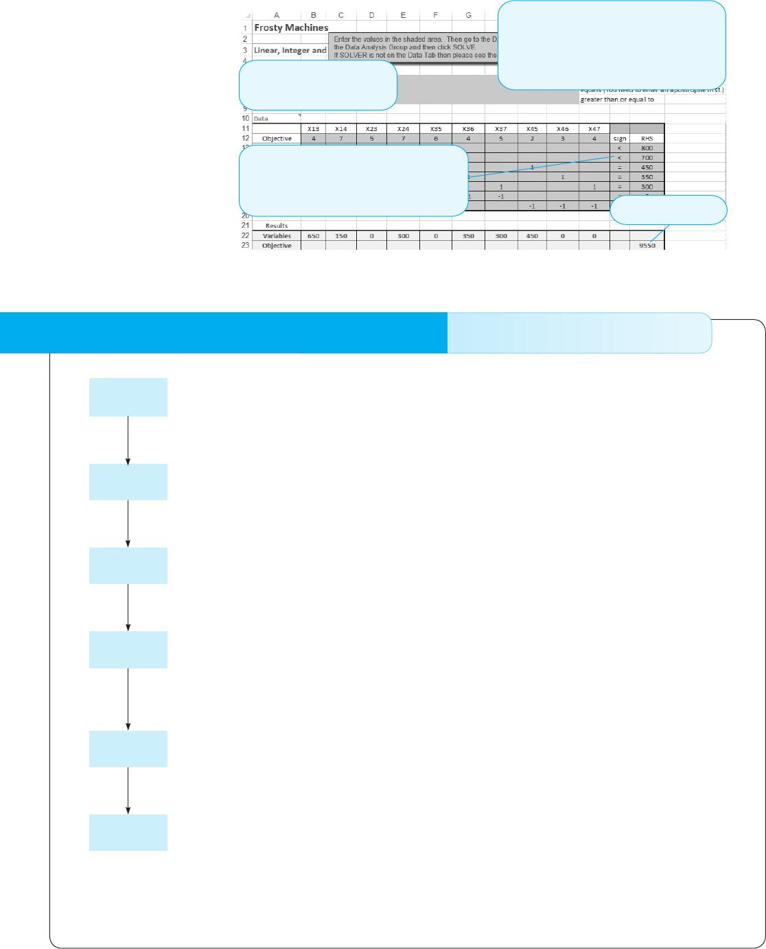
The solution found using Solver in Excel 2013 and Excel QM is shown in Program 9.5. The
total cost is $9,550 by shipping 650 units from Toronto to Chicago, 150 units from Toronto to
Buffalo, 300 units from Detroit to Buffalo, 350 units from Chicago to Philadelphia, 300 units
from Chicago to St. Louis, and 450 units from Buffalo to New York City.
Table 9.3 Frosty Machine Transshipment Data
to
FroM chicago BuFFalo
neW york
city PhilaDelPhia St. louiS SuPPly
Toronto $4 $7 — — — 800
Detroit $5 $7 — — — 700
Chicago — — $6 $4 $5 —
Buffalo — — $2 $3 $4 —
Demand — — 450 350 300
Special transshipment
constraints are used in the
linear program.
M09_REND9327_12_SE_C09.indd 351 10/02/14 1:28 PM
Copyright 2015. Pearson.
All rights reserved. May not be reproduced in any form without permission from the publisher, except fair uses permitted under U.S. or applicable copyright law.
EBSCO Publishing : eBook Collection (EBSCOhost) – printed on 7/26/2020 2:00 PM via UNIVERSITY OF JOHANNESBURG
AN: 1419013 ; Render, Barry, Stair, Ralph M, Hanna, Michael E., Hale, Trevor S..; Quantitative Analysis for Management, Global Edition
Account: s6390179.main.eds
352 Chapter 9 • transportation, assignment, and network models
From Excel QM ribbon, select Menu
(Alphabetical or By Chapter). Select Linear
Programming from the drop-down menu.
Then ll in the number of constraints (7),
the number of variables (10), select
Minimize, and click OK.
The solution is here.
After entering the data,
click the Data tab and select
Solver. Then click Solve.
When the worksheet opens, ll in the
table with the coefcients for the objective
function and the constraints. Type over
the “,” symbol to change it.
Program 9.5
Excel QM Solution
to Frosty Machine
Transshipment Problem
in Excel 2013
Defining the Problem
The sugar market has been in a crisis for over a decade. Low sugar prices and decreasing demand have
added to an already unstable market. Sugar producers needed to minimize costs. They targeted the largest
unit cost in the manufacturing of raw sugar contributor—namely, sugar cane transportation costs.
Developing a Model
To solve this problem, researchers developed a linear program with some integer decision variables
(e.g., number of trucks) and some continuous (linear) variables and linear decision variables (e.g., tons of
sugar cane).
acquiring input Data
In developing the model, the inputs gathered were the operating demands of the sugar mills involved, the
capacities of the intermediary storage facilities, the per-unit transportation costs per route, and the pro–
duction capacities of the various sugar cane fields.
testing the Solution
The researchers involved first tested a small version of their mathematical formulation using a spreadsheet.
After noting encouraging results, they implemented the full version of their model on a large capacity
computer. Results were obtained for this very large and complex model (on the order of 40,000 decision
variables and 10,000 constraints) in just a few milliseconds.
analyzing the results
The solution obtained contained information on the quantity of cane delivered to each sugar mill, the field
where cane should be collected, and the means of transportation (by truck, by train, etc.), and several
other vital operational attributes.
implementing the results
While solving such large problems with some integer variables might have been impossible only a decade
ago, solving these problems now is certainly possible. To implement these results, the researchers worked
to develop a more user-friendly interface so that managers would have no problem using this model to
help make decisions.
Source: Based on E. L. Milan, S. M. Fernandez, and L. M. Pla Aragones. “Sugar Cane Transportation in Cuba: A Case Study,”
European Journal of Operational Research, 174, 1 (2006): 374–386.
MODeling in the reAl WOrlD Moving sugar Cane in Cuba
Defining
the Problem
Developing
a Model
Acquiring
Input Data
Testing the
Solution
Analyzing
the Results
Implementing
the Results
M09_REND9327_12_SE_C09.indd 352 10/02/14 1:28 PM
EBSCOhost – printed on 7/26/2020 2:00 PM via UNIVERSITY OF JOHANNESBURG. All use subject to https://www.ebsco.com/terms-of-use
9.5 maximal-Flow problem 353
9.5 Maximal-Flow Problem
The maximal-flow problem involves determining the maximum amount of material that can
flow from one point (the source) to another (the sink) in a network. Examples of this type of
problem include determining the maximum number of cars that can flow through a highway
system, the maximum amount of a liquid that can flow through a series of pipes, the maxi–
mum number of cell-phone calls that can pass through a series of cell towers, and the maximum
amount of data that can flow through a computer network.
To find the maximal flow from the source or start of a network to the sink or finish of that
network, two common methods are used: linear programming and the maximal-flow technique.
We will begin by presenting an example and demonstrating the use of linear programming for
this type of problem.
Example
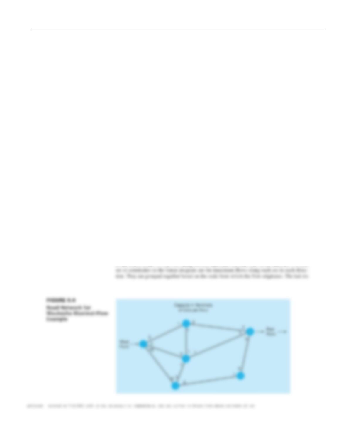
Waukesha, a small town in Wisconsin, is in the process of developing a road system for the
downtown area. Bill Blackstone, one of the city planners, would like to determine the maximum
number of cars that can flow through the town from west to east. The road network is shown in
Figure 9.4. The streets are indicated by their respective arcs. For example, the arc from node 1
to node 2 is arc 1–2. The arc in the reverse direction (from node 2 to node 1) is arc 2–1. The
numbers by the nodes indicate the maximum number of cars (in hundreds of cars per hour) that
can flow from the various nodes along the respective arcs. The maximum flow along arc 1–2 is 3,
while the flow along arc 1–3 is 10. The city planners would like to know the capacity of the cur–
rent road system in the west to east direction.
The maximal-flow problem can be modeled as a linear program. This type of problem may
be viewed as a special type of transshipment problem with one source, one destination, and a
number of transshipment points. The number shipped through the network would be called the
flow. The objective is to maximize the flow through the network. There are two types of con–
straints. The first set of constraints restricts the amount of flow on any arc to the capacity of that
arc. The second set of constraints indicates that the amount of flow out of a node will equal the
amount of flow into that node. These are the same as the transshipment constraints in the trans–
shipment problem.
The variables are defined as:
X
ij
=flow
from
node
i
to
node
j
One additional arc will be added to the network, and this arc will go from the sink (node 6) back
M09_REND9327_12_SE_C09.indd 353 10/02/14 1:28 PM
M09_REND9327_12_SE_C09.indd 354 10/02/14 1:28 PM
M09_REND9327_12_SE_C09.indd 355 10/02/14 1:28 PM
M09_REND9327_12_SE_C09.indd 356 10/02/14 1:28 PM
M09_REND9327_12_SE_C09.indd 357 10/02/14 1:28 PM
M09_REND9327_12_SE_C09.indd 358 10/02/14 1:28 PM
M09_REND9327_12_SE_C09.indd 359 10/02/14 1:28 PM
M09_REND9327_12_SE_C09.indd 360 10/02/14 1:28 PM