Jessica Wachter Notes for Finance 604
Topic 4: Applications to Equity Valuation
(a) Using Present Value Methods to Value Equity
We’ve determined the value of fixed income securities (bonds) using present value methods.
Can we apply the same to stocks?
Definition Equity: The residual claim on the assets of a corporation.
Namely, equity is what is left after the bondholders have been paid. If you own equity in a
company, you are a partial owner of that company. Another word for equity is common
stock.
1. Dividend.
2. Capital Gain (or price appreciation).
Notation:
•P0= Current price per share.
•P1= Price per share next year.
•D1= Dividend per share next year.
Prices are ex-dividend (namely, P0is the price just after the current dividend has been
paid).
Holding period return (HPR):
r=V1−V0
V0
=D1+P1−P0
P0
=D1
P0
+P1−P0
P0
The term D1/P0is the dividend-yield. The term (P1−P0)/P0is the percent price
appreciation (or percent capital gain).
We can invert the formula for rto write the price today given D1and P1:
1 + r=D1+P1
P0
1

Jessica Wachter Notes for Finance 604
so that
P0=D1+P1
1 + r.
This also makes sense based on present-value reasoning. Price today is the present
discounted value of payments one period from now.
However, this formula is not satisfying – how do we know what P1is? We could apply the
same formula to P1and find:
P1=D2+P2
1 + r.
Substituting this in, we find:
P0=D1
1 + r+D2
(1 + r)2+P2
(1 + r)2.
More generally:
Pt=D1
1 + r+D2
(1 + r)2+· · · +Dt
(1 + r)t+Pt
(1 + r)t.
Under reasonable conditions for Pt(where rate of growth of Pis less than rfor a
sufficiently high period t) we can take limits to find:
Pt=D1
1 + r+D2
(1 + r)2+· · · +Dt
(1 + r)t+· · ·
This is a formula for the price given the (possibly infinite) stream of future dividends.
Note: this is price per share. But we can also value the entire firm if given total dividends.
Note: “dividends” can be any cash flow from the corporation to investors. If the company
liquidates, the liquidation value is treated as one big dividend. If another company buys the
shares for cash, that is also a “dividend” in this analysis. The bottom line: we value equities
the same way we value any other asset – we discount the future stream of cash flows.
In principle, this sounds simple. However, there is an important difference between bonds
and equities: equity cash flows are uncertain. For bonds, remember that cash flows are
fixed – bonds are fixed-income securities. However, for equities, while we can estimate
dividends, we don’t know what they will be for sure.
Instead, we use expected dividends in the numerator. In the denominator, the rwe use will
in general not be the same ras for bonds. In the second half of the course, we will pay a
lot of attention to finding the appropriate r. For now, we take rto be the rate of return on
an investment of comparable risk to the firm’s dividend process. Typically (for reasons we
will see), this will be higher than the rate available on bonds or at the bank.
We are about to get into the specifics of valuing equity. The approach of valuing equity
through its cash flows takes some getting used to, and you may find yourself wondering “do
2

Jessica Wachter Notes for Finance 604
people really value equity this way?” YES! As we will learn, the principle of using multiples
(such as the price-earnings ratio) to value equity all comes down to thinking of equity as a
stream of future cash flows. This approach is the standard in the financial industry.
(b) Applying Infinite-Horizon Formulas
1. Constant Dividend Growth
How do we determine expected dividends? We build a model. Our first model will be
simple, but nonetheless will capture the important feature that equity is a long-lived
asset in which the cash flows (dividends) grow over time.
Let D1be expected dividends next year, and gthe growth rate in expected
dividends. Then the dividend stream is as follows:
D2=D1(1 + g)
D3=D1(1 + g)2
.
.
..
.
.
Dt=Dt(1 + g)t−1
.
.
..
.
.
And the price today is
P0=D1
1 + r+D1(1 + g)
(1 + r)2+· · · +D1(1 + g)t−1
(1 + r)t+· · ·
By applying the formula for a growing perpetuity, we arrive at
P0=D1
r−g.
Recall that the formula for the growing perpetuity assumes r > g.
Example Assume: D1=$3, g=10%, and r=15%. Then:
P0=3
.15 −.1= $60.
An aside: you may say – plenty of companies grow at a rate >15%! Often, you hear
forecasts of 50% growth, but not of 50% growth rates that last forever! It may be
unrealistic to assume a constant growth rate forever for some companies. Companies
typically grow quickly when they are young and more slowly when they get old.
3
Jessica Wachter Notes for Finance 604
2. OPTIONAL: Differential Growth
Example Consider a company whose dividends are expected to grow at 15% for the
next five years, and 10% after that. If the dividend next year is expected to be
$2.3/share and the discount rate is 15%, what should price/share be today?
More generally: a company grows for Nyears at g1, then at g2. Assume r > g2.
Phase I :
D1=D1
D2=D1(1 + g1)
.
.
.
DN=D1(1 + g1)N−1.
Phase II :
DN+1 =DN(1 + g2) = D1(1 + g1)N−1(1 + g2)
DN+2 =DN(1 + g2)2=D1(1 + g1)N−1(1 + g2)2
.
.
.
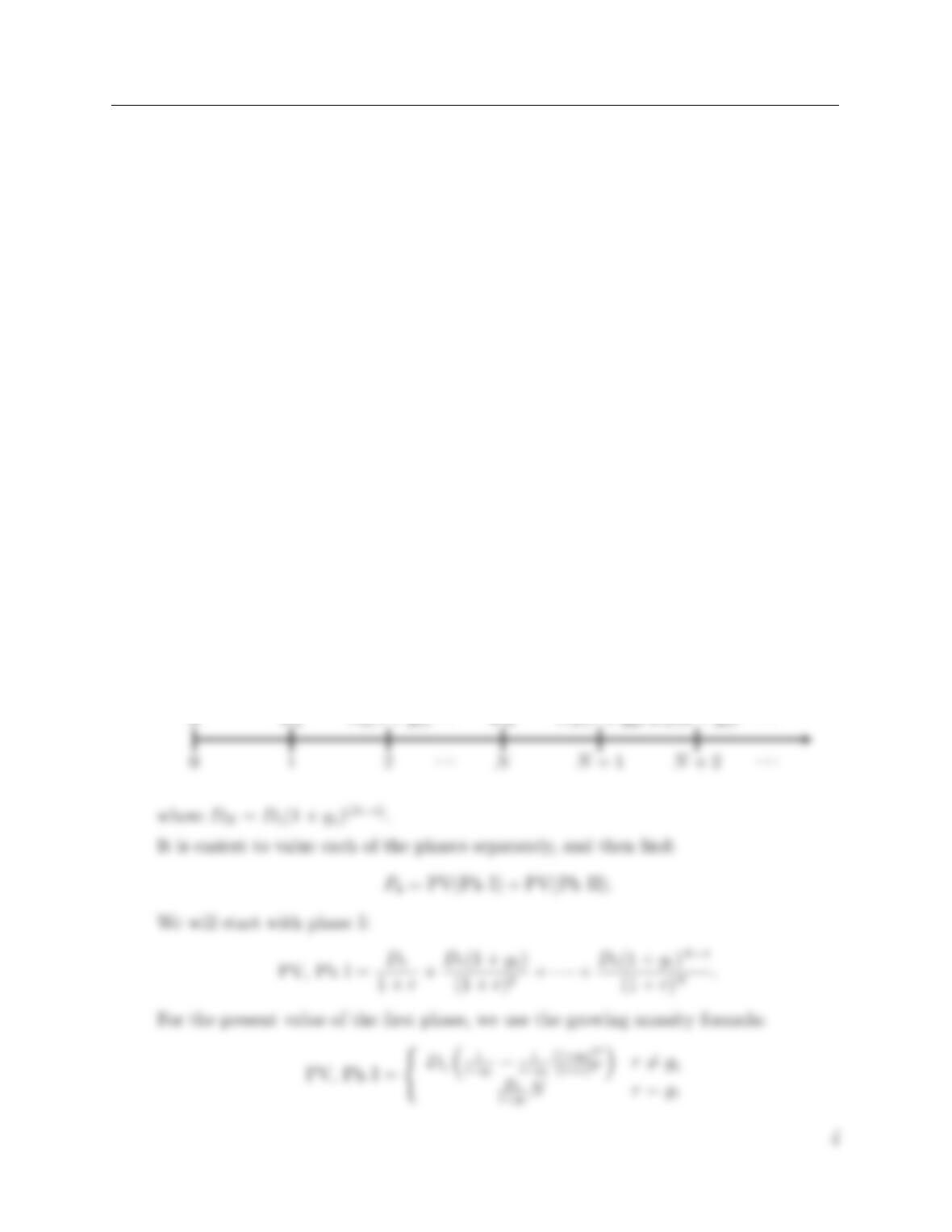
To illustrate the cash flows:
. . . . . .