THEORY OF PRODUCTION AND COST IN THE
SHORT AND THE LONG RUN
INTENDED LEARNING OUTCOMES
1. Describe the production function in the short-run.
2. Interpret the short-run total costs.
3. Determine the relation between short-run costs and production.
4. Choose the optimal combination of inputs.
5. Analyze the long-run cost curve.
6. Distinguish the relationship between short-run and long-run costs
A firm is an entity concerned with the purchase and employment of resources in the production
of various goods and services. It will be assumed throughout the course of our discussion that the firm
aims to maximize its output with the use of resources that are substitutable to a certain degree.
Furthermore, the firm is a price taker in terms of the resources it uses.
PRODUCTION FUNCTION
Production is the creation of goods and services using the inputs of production. The physical
relationship between the inputs and outputs of goods and services at a given period of time, ceteris
paribus is called a production function and is expressed in the mathematical form:
Q = f(x)
where Q = output
x = inputs
f= production process
Output refers to the goods and services that have been created using the production inputs.
Inputs of production refer to the factors of production which include land, labor, capital, and
entrepreneurship (see detailed discussion in the introductory part). Inputs are classified as follows:
1. Fixed inputs – they are those that remain regardless of the volume or quantity of production.
This means that whether you produce or not, the factors of production is unchanged.
2. Variable inputs – these are those that vary in accordance to the volume or quantity of
production. If there is no production; then, there is no variable inputs.
For instance, a rice farmer’s production function may include several possible combinations of
land (fixed input), labor and seeds (variable inputs) in the production of varying amounts of rice. In a
6
similar way, the production function of a fish-cracker maker may include combinations of machinery
(fixed input) and workers (variable) in the production of varying amounts of fish-crackers.
PRODUCTION ANALYSIS WITH ONE VARIABLE INPUT
The Law of Diminishing Returns
It states that when successive units of the variable input is combined with a fixed input, the total
product (TP) or output (Q) will increase, but beyond some points the resulting increases in output will
become smaller and smaller. The following concepts will be used in analyzing this principle.
Total Product (TP). It refers to the total production or output (Q).
Marginal (Physical) Product (MP). It is the additional output produced by employing one
additional unit of input (X) holding the level of usage of all other inputs constant.
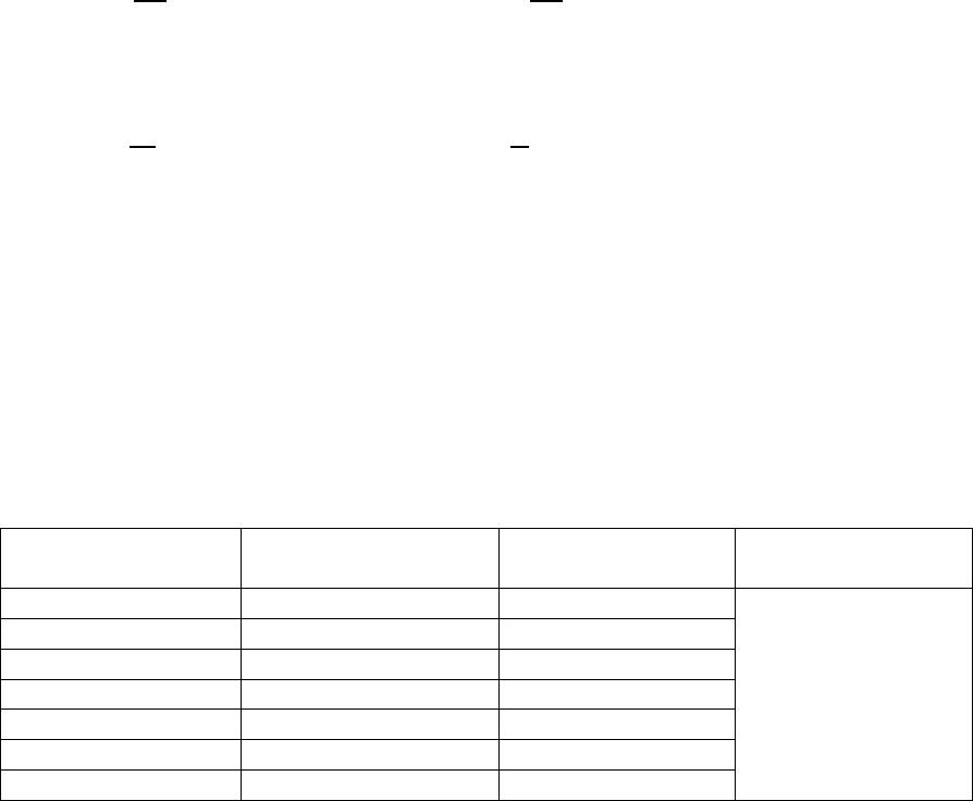
MP = ∆Q or using Q to denote TP; thus, MP = ∆Q
∆x ∆x
Average (Physical) Product (AP). It is the output produced per unit of the input.
AP = TP or using Q to denote TP; thus, AP = Q
x x
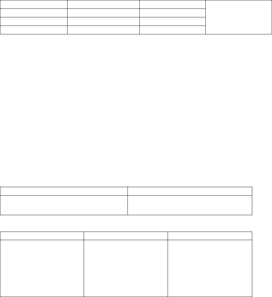
Table 6.1 shows the production schedule of a rice farmer given the variable input – workers.
Total, average and marginal production in this case is measured in physical units (cavans). Notice that as
more workers are employed, Total Product increases although at some point beyond the 8th worker,
production has declined. Increases in the production for rice as an additional worker is hired are reflected
by the Marginal product column. We can observe that each additional worker from workers 1 to workers
2 to the 7th worker, yield positive increases to production. However, the increment to production is
diminishing! This scenario explains the law of diminishing returns at work. This means that we cannot
produce every rice needs in our country in single piece of land. Further, Table 6.1 is graphically illustrated
in Figure 6.1.
Table 6.1 Total product (in cavans) schedule of rice production with workers as variable input (x).
Units of workers (x)
Total product (TP) or
Output (Q)
Average product
(AP)
Marginal Product
(MP)
0
0
–
5
10
14
15
11
6
3
1
5
5.0
2
15
7.5
3
29
9.7
4
44
11.0
5
55
11.0
6
61
10.2
7
64
9.1
0
-2
-3
8
64
8.0
9
62
6.9
10
59
5.9
Three Stages of Production
The stage 1 of the production process is characterized by an increasing AP. In Figure 5.1, this
occurs from the origin (0) up to x=4. The increasing AP is explained by specialization and teamwork
gained from an additional X. Moreover, at this stage the fixed input is grossly underutilized. The point of
equality between AP and MP serves as the boundary between stages 1 and 2 of the production process.
At this point of intersection (MP=AP), it is noticeable that the AP has reached its maximum value.
The stage 2 of the production process corresponds to the range of x from 5 up to 8. The end point
of stage 2 corresponds to the point of maximum output on the TP curve. This maximum TP happens
when the MP is equal to zero (MP=0). This serves as the boundary between stages 2 and 3 of the
production process. At this level, MP and AP are declining.
The stage 3 of the production process encompasses the range of x over which the total product
is declining (which corresponds to a negative MP). Stage 3 occurs when x exceeds 8 where the crowding
out effects overwhelms any output attributable to additional workers. In order to identify the stages of
production the condition of boundaries should be satisfied as showed in table 6.2 and figure 6.1.
Table 6.2 Condition of the Boundaries
Boundary I
Boundary II
1. AP is at maximum
2. AP = MP
1. TP is at maximum
2. MP = 0
Table 6.3 Characteristics of the Three Stages of Production
Stage I
Stage 2
Stage 3
1. TP is increasing at
faster rate
2. AP and MP are
increasing
3. AP < MP
4. MP > 0 (positive)
1. TP is increasing at
slower rate
2. AP and MP are
decreasing
3. AP > MP
4. MP > 0 (positive)
1. TP is decreasing
2. AP and MP are
decreasing
3. AP > MP
4. MP < 0 (negative)
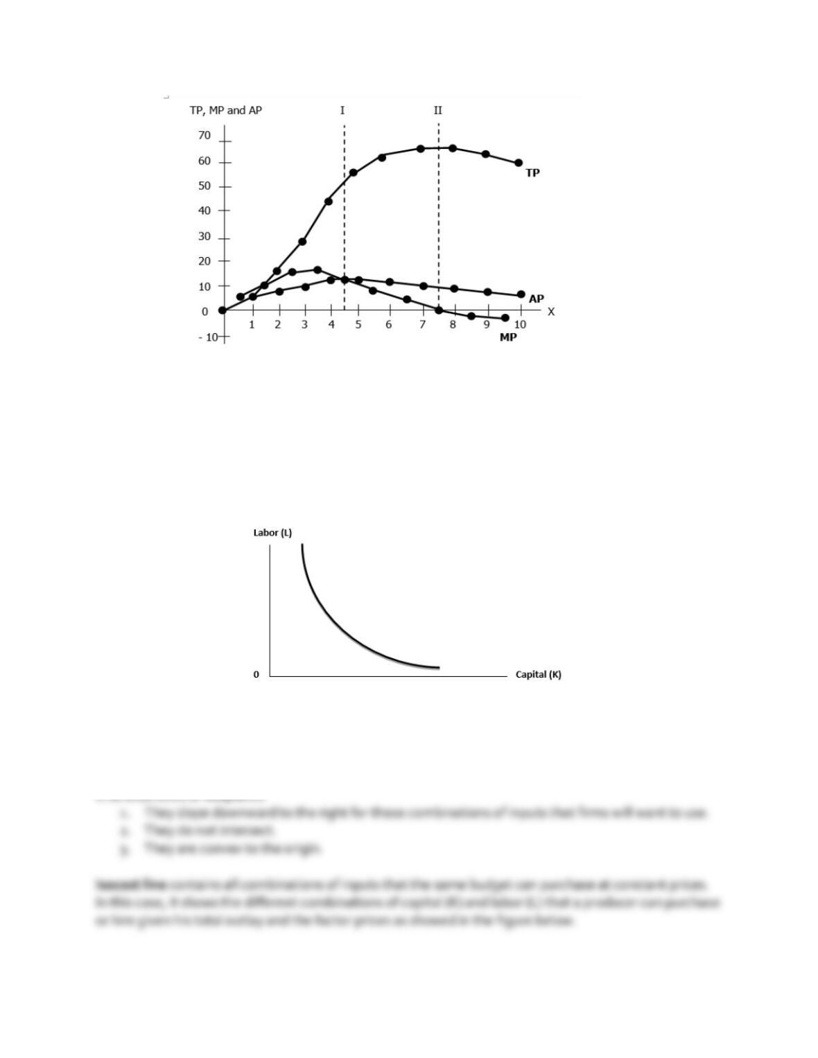
Figure 6.1 Graphical Illustration of the 3 stages of production.
PRODUCTION ANALYSIS WITH TWO VARIABLE INPUTS
Production Isoquant and Isocost
Isoquant represents the various combinations of two inputs that can be used to produce the same
level of output. In this case, an isoquant shows the different combinations of capital (K) and labor (L)
which yield the same level of output as showed in the figure below.
Figure 6.2 Isoquant Curve showing Labor and Capital.