The Theory of Interest – Solutions Manual
46
Chapter 5
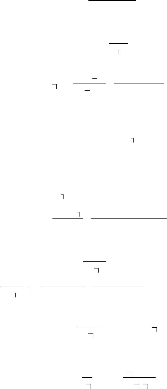
1. The quarterly interest rate is .06/ 4 .015j
=
=. The end of the second year is the end of
the eighth quarter. There are a total of 20 installment payments, so
20 .015
1000
Ra
=
and using the prospective method
(
)
12 .015
812 .015
20 .015
1000 1000 10.90751 $635.32.
17.16864
pa
BRa a
== = =
2. Use the retrospective method to bypass having to determine the final irregular
payment. We then have
()
()
()()()
5
55.12
10,000 1.12 2000
10,000 1.76234 2000 6.35283
$4918 to the nearest dollar.
r
Bs=−
=−
=
3. The quarterly interest rate is .10/ 2 .025
j
=
=. Applying the retrospective method we
have
()
4
44
1
r
j
BL j Rs=+− and solving for L
()
()
44
4
12,000 1500 4.15252
1.10381
1
$16,514 to the nearest dollar.
r
j
BRs
Lj
++
==
+
=
4. The installment payment is
12
20,000
Ra
= and the fourth loan balance prospectively is
(
)
(
)
82
412 3
8
12
20,000 20,000 1 20,000 1 2 $17,143 to the nearest dollar.
112
pv
Ba
av
−
−
−−
== = =
−−
5. We have
515
20
20,000 and .
P
RBRa
a
==
The revised loan balance at time 7t
=
is
()
2
75
1,
p
BB i
′=+ since no payments are
made for two years. The revised installment payment thus becomes
(
)
2
715
13 20 13
1
20,000 .
a i
B
Raaa
+
′==
The Theory of Interest – Solutions Manual Chapter 5
47
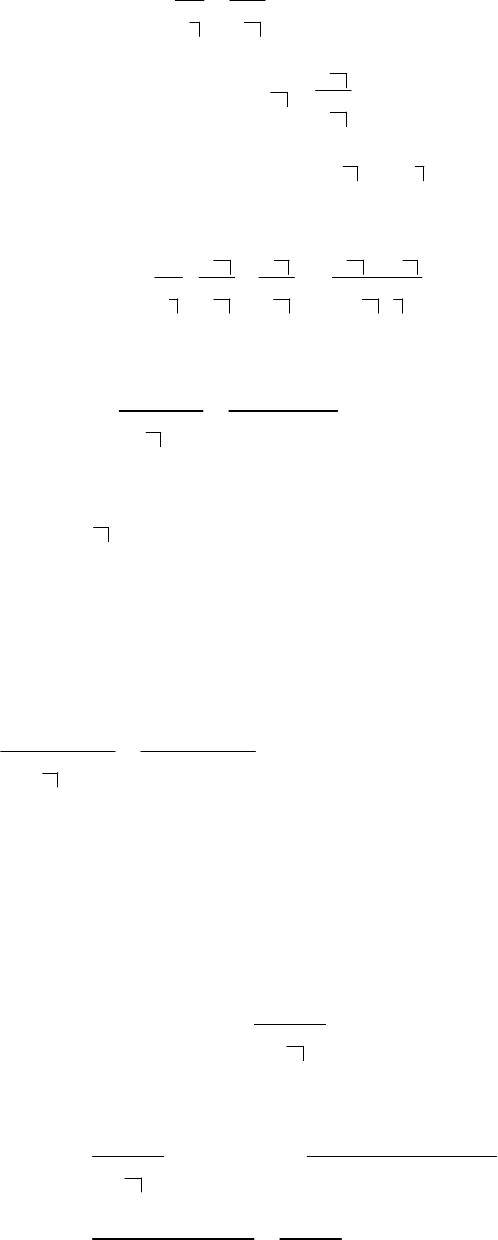
6. The installment payment is
25
1
n
L
Raa
== . Using the original payment schedule
20
520
25
pa
BRa a
==
and using the revised payment schedule 515 5
p
BRaKa=+. Equating the two
and solving for K we have
20 15 20 15
525 25 255
1.
aa aa
Kaa a aa
−
⎛⎞
=−=
⎜⎟
⎝⎠
7. We have
15 .065
150,000 150,000 15,952.92
9.4026689
Ra
== =
and
(
)
(
)
510 .065 15,952.92 7.1888302 114,682.83
p
BRa==.
The revised fifth loan balance becomes
5114,682.83 80,000 194,682.83B′=+=
and the revised term of the loan is 15 5 7 17.n
′
=
−+= Thus, the revised installment
payment is
17 .075
194,682.83 194,682.83 $20,636 to the nearest dollar.
9.4339598
Ra
′===
8. The quarterly interest rate is .12/ 4 .03.j
=
= Directly from formula (5.5), we have
()
15
20 6 1
6.03
1000 1000 1.03 $641.86.Pv −
−+
== =
9. The installment payment is
20
10,000
Ra
=
and applying formula (5.4) we have
()
(
)
(
)
()
()()
10
20 11 1
11 20
20
10
10
10 10
10,000 10,000 .1 1
11
1000 1 1000 .
1
11
v
Iv
av
v
v
vv
−+ −
=−=
−
−
==
+
−+
The Theory of Interest – Solutions Manual Chapter 5
48
10. The quarterly interest rate is .10/ 4 .025j
=
=. The total number of payments is
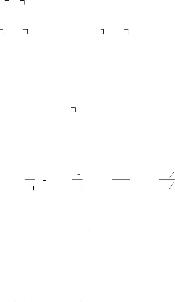
54 20n=×= . Using the fact that the principal repaid column in Table 5.1 is a
geometric progression, we have the answer
()()()()()
()
()
13 14 15 16 17
18 13
100 1 1 1 1 1
100 100 22.38635 15.14044 $724.59.
iiiii
ss
⎡⎤
+++++++++
⎣⎦
=−= − =
11. (a) We have 6
46 10
pi
ij
Ba va=+ so that
(
)
6
54
6 10
i
ij
IiBia va=⋅ = + .
(b) After 10 years, the loan becomes a standard loan at one interest rate. Thus applying
formula (5.5)
20 15 1 6
15 .
j
j
P
vv
−+
=
=
12. After the seventh payment we have 713
p
Ba=. If the principal 20 8 1 13
8
P
vv
−+
== in the
next line of the amortization schedule is also paid at time 7t
=
; then, in essence, the
next line in the amortization schedule drops out and we save 13
1v
−
in interest over the
life of the loan. The loan is exactly prepaid one year early at time 19t=.
13. (a) The amount of principal repaid in the first 5 payments is
523
5
05 5 10
549
10 10
11
11 1.4.
11
pa
Lv
BBLB L a L L L L
aav
⎛⎞⎛ ⎞
−−
⎛⎞ ⎛ ⎞
−=− =− = − = − = − =
⎜⎟
⎜⎟ ⎜⎟
⎜⎟ −−
⎝⎠
⎝⎠
⎝⎠ ⎝ ⎠
(b) The answer is
()( )
5
5
3
1.4.9.
2
BiLL L+=− =
14. We are given
(
)
(
)
28 14
822
1 135 and 1 108.IR v I R v=−= =−=
Taking the ratio
814
814
22
1 135
11.25
1 108
Ivv
Iv
−
==+==
−
so that
14 .25v=.
The Theory of Interest – Solutions Manual Chapter 5
Now, we can solve for R
14
108 108 144.
1.75
Rv
===
−
Finally,
()
()
.5
7
29 1 144 1 .25 $72.IRv ⎡⎤
=−= − =
⎣⎦
15. We have
10
1000
L
a
=
.
and using the column total from Table 5.1
(
)
10
1000 10
L
a=−
Equating the two we have 10 5a
=
and solving for the unknown rate of interest using a
financial calculator, we have 15.0984i
=
%. Thus, the answer is
(
)
(
)
1.150984 5000 $754.95.IiL== =