Learning Module on Macroeconomics Page | 1
ECONOMIC GROWTH THEORY: THE
ECONOMY IN THE VERY LONG RUN
INTENDED LEARNING OUTCOMES
By the end of the learning experience, students must be able to:
1. Explain and articulate the Economic Growth Theories and how national income grows across
countries
2. Distinguish how savings, population growth, and technological progress affect the level of
an economy’s output and its growth overtime
3. Broaden ones analysis so as to describe changes in the economy among nations over the
world overtime
4. Appraise why some economies grow faster than others
A. THE ACCUMULATION OF CAPITAL
Our primary task in this chapter and the next is to develop a theory of economic growth called
the Solow Growth Model
The Solow growth model shows how savings, population growth, and technological progress
affect the level of an economy’s output and its growth over time. In this chapter we analyze the
roles of saving and population growth.
The Solow growth model is designed to show how growth in the capital stock, growth in the
labor force, and advances in technology interact in an economy as well as how they affect a
nation’s total output of goods and services. We will build this model in a series of steps. Our
first step is to examine how the supply and demand for goods determine the accumulation of
capital. In this first step, we assume that the labor force and technology is fixed. We then relax
these assumptions by introducing changes in the labor force in this chapter later.
The Supply and Demand of Goods
The supply and demand for goods played a central role in our static model of the closed
economy. The same is true for the Solow Model. By considering the supply and demand for
goods, we can see what determined how much output is produced at any given times and how
this output is allocated among alternative uses.
Solow Growth Model is named after economist Robert Solow and was developed in the 1950s
and 1960s. In 1987 Solow won the Nobel Prize in economics for his work on economic growth.
The Supply of Goods and the Production Function The supply of goods in the Solow Model is
based on the production function, which states that output depends on the capital stock and
the labor force
= ,
11
Learning Module on Macroeconomics
The Solow growth model assumes that the production function has constant returns to scale.
Recall that a production function has a constant returns to scale if
Production
functions with constant return to scale allow us to analyze all quantities in the
economy relative to the size of the labor force. To see that this is true, set z = 1/L in the
preceding equation to obtain
=
This
equation shows that the amount of output per worker Y/L is a function of the amount of
capital per worker K/L (The number 1 is constant and thus can be ignored). The assumption of
constant returns to scale implies that the size of the economy
workers —
does not affect the relationship between output per worker and capital per worker.
Because the size of the economy does not matter, it will prove convenient to denote all
quantities in per worker terms. We designate quan
y = Y/L is output per worker
production function as:
=
Where we define
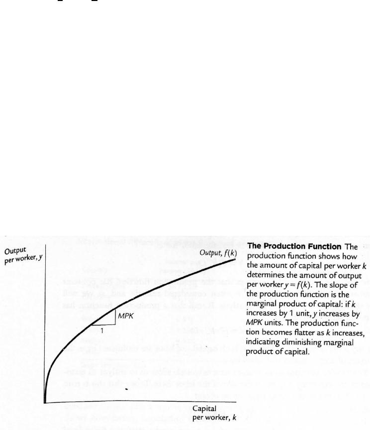
FIGURE 11-1
The slope of the production function shows how much extra output a worker produces when
given an extra unit of capital.
Mathematically, we write
Note that in
Figure 11
flatter, indicating that the production function exhibits diminishing marginal product of capital.
When k is low, the average worker has only a little capital to work with, s
capital is very useful and produces a lot of additional output. When k is high, the average
worker has a lot of capital already, so an extra unit increases production only slightly.
Learning Module on Macroeconomics
The Solow growth model assumes that the production function has constant returns to scale.
Recall that a production function has a constant returns to scale if
= , for any positive number z
functions with constant return to scale allow us to analyze all quantities in the
economy relative to the size of the labor force. To see that this is true, set z = 1/L in the
preceding equation to obtain
,
equation shows that the amount of output per worker Y/L is a function of the amount of
capital per worker K/L (The number 1 is constant and thus can be ignored). The assumption of
constant returns to scale implies that the size of the economy
does not affect the relationship between output per worker and capital per worker.
Because the size of the economy does not matter, it will prove convenient to denote all
quantities in per worker terms. We designate quan
tities per worker with lowercase letters, so
y = Y/L is output per worker
, and
k = K/L is capital per worker
production function as:
,1. Figure 11-
1 illustrates this production function
The slope of the production function shows how much extra output a worker produces when
given an extra unit of capital.
This amount is the marginal product of capital MPK.
Mathematically, we write
Figure 11
–
1, as the amount of capital increases, the production function becomes
flatter, indicating that the production function exhibits diminishing marginal product of capital.
When k is low, the average worker has only a little capital to work with, s
capital is very useful and produces a lot of additional output. When k is high, the average
worker has a lot of capital already, so an extra unit increases production only slightly.
Page | 2
The Solow growth model assumes that the production function has constant returns to scale.
Recall that a production function has a constant returns to scale if
functions with constant return to scale allow us to analyze all quantities in the
economy relative to the size of the labor force. To see that this is true, set z = 1/L in the
equation shows that the amount of output per worker Y/L is a function of the amount of
capital per worker K/L (The number 1 is constant and thus can be ignored). The assumption of
constant returns to scale implies that the size of the economy
— as measured by the number of
does not affect the relationship between output per worker and capital per worker.
Because the size of the economy does not matter, it will prove convenient to denote all
tities per worker with lowercase letters, so
k = K/L is capital per worker
. We can then write the
1 illustrates this production function
.
The slope of the production function shows how much extra output a worker produces when
This amount is the marginal product of capital MPK.
1, as the amount of capital increases, the production function becomes
flatter, indicating that the production function exhibits diminishing marginal product of capital.
When k is low, the average worker has only a little capital to work with, s
o an extra unit of
capital is very useful and produces a lot of additional output. When k is high, the average
worker has a lot of capital already, so an extra unit increases production only slightly.
Learning Module on Macroeconomics Page | 3
The Demand for Goods and the Consumption Function The demand for goods in the Solow
model comes from consumption and investment. In other words, output per worker y is divided
between consumption per worker c and investment ί
This equation is the per-worker version of the national income accounts identity for an
economy. Notice it omits G and NX for we assume a closed economy.
The Solow model assumes that each year people save a fraction s of their income and consume
a fraction (1 – s). We can express this idea with the following consumption function:
Where s is saving rate, it is a number between 0 and 1. For now, we just take the saving rate s as
given.
To see what this consumption function implies for investment, substitute (1 – s) y for c in the
national income accounts identity:
Rearrange the terms to obtain
This equation shows that investment equals saving. Thus, the rate of saving s is also the
fraction of output devoted to investment.
We have now introduced the 2 main ingredients of the Solow model —– the production function
and the consumption function which describes the economy at any moment in time. For any
given capital stock k, the production function y =f(k) determines how much output the
economy produces, and the saving rate, s determine the allocation of that output between
consumption and investment.
Growth in the Capital Stock and the Steady State
At any moment, the capital stock is a key determinant of the economy’s output, but the capital
stock can change over time, and those changes can lead to economic growth. In particular, two
forces influence the capital stock: investment and depreciation. Investment is expenditure on
new plant and equipment it causes the capital stock to rise. Depreciation is the wearing out of
old capital, and it causes the capital stock to fall.worker.
As we have already noted, investment per worker ί equals sy. By substituting the production
function for y, we can express investment per worker as a function of the capital stock per
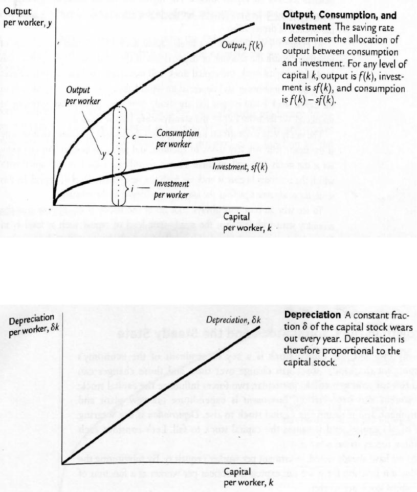
This equation relates the existing stock of capital k to the accumulation of new capital ί. Figure
11-2 shows this relationship. Figure 11-2 illustrates how, for an y value of k, the amount of
output is determined by the production function f(k), and the allocation of that output between
consumption and investment is determined by the saving rate, s
To incorporate depreciation into the model, we assume that a certain fraction of the capital
stock wears out each year. Here (the lowercase Greek letter delta) is called the depreciation
Learning Module on Macroeconomics
rate. For example,
(
= 0.04). The amount of capital that depreciates each year is
amount of depreciation depends on the capital stock.
FIGURE 11-2
FIGURE 11-3
We can express the impact of investment and depreciation on the capital stock with this
equation:
Changes in capital stock = Investment
∆
Where Δk is the change of the capital stock between one year and the next. Because
investment ί equals
Learning Module on Macroeconomics
rate. For example,
if capital lasts an average of 25 years then the depreciation rate is 4%/year
= 0.04). The amount of capital that depreciates each year is
amount of depreciation depends on the capital stock.
We can express the impact of investment and depreciation on the capital stock with this
Changes in capital stock = Investment
–
Depreciation
∆
Where Δk is the change of the capital stock between one year and the next. Because
investment ί equals
, we can write this as
Page | 4
if capital lasts an average of 25 years then the depreciation rate is 4%/year
= 0.04). The amount of capital that depreciates each year is
k. Figure 11-3 shows how the
We can express the impact of investment and depreciation on the capital stock with this
Depreciation
Where Δk is the change of the capital stock between one year and the next. Because
Learning Module on Macroeconomics
∆
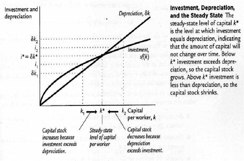
Figure 11-
4 graphs the terms of this equation
levels of capital stock k. The higher the capital stock, the greater the amounts of output and
investment. Yet the higher the capital stock, the greater also the amount
As Figure 11-
4, shows there is a single capital stock k
equals the amount of depreciation. If the economy finds itself at this level of capital stock, the
capital stock will not change because the 2
just balance.
FIGURE 11-4
That is at k
*
,
∆k = 0, so the capital stock k and output f(k) are steady over time. We therefore
call k
*
the steady-
state level of capital
The steady state is significant because
Regardless of the level of capital with which the economy begins, it ends up with the steady
state level of capital. In this sense,
the economy.
To see why an economy always ends up at the steady state, suppose that the economy starts
with less than the steady
level of investment exceeds the amount of depreciation. Over time, the capital stock will rise
and will continue to rise
Similarly, suppose that t
such as level k
2
. In this case, investment is less than depreciation: capital is wearing out faster
than it is being replaced. The capital stock will fall, again approaching the steady
Once the capital stock reaches the steady state, investment equals depreciation, and there is
no pressure for the capital stock to either increase or decrease.
Learning Module on Macroeconomics
4 graphs the terms of this equation
–
investment and depreciation
levels of capital stock k. The higher the capital stock, the greater the amounts of output and
investment. Yet the higher the capital stock, the greater also the amount
4, shows there is a single capital stock k
*
at which the amount of investment
equals the amount of depreciation. If the economy finds itself at this level of capital stock, the
capital stock will not change because the 2
forces acting on it
—-
∆k = 0, so the capital stock k and output f(k) are steady over time. We therefore
state level of capital
.
The steady state is significant because
an economy at the steady state will stay there.
Regardless of the level of capital with which the economy begins, it ends up with the steady
state level of capital. In this sense,
the steady state represents the lo
To see why an economy always ends up at the steady state, suppose that the economy starts
with less than the steady
–
state level of capital, such as level k
level of investment exceeds the amount of depreciation. Over time, the capital stock will rise
and will continue to rise
— along with output f(k) —
until it approaches the steady state k
Similarly, suppose that t
he economy starts with more than the steady
. In this case, investment is less than depreciation: capital is wearing out faster
than it is being replaced. The capital stock will fall, again approaching the steady
Once the capital stock reaches the steady state, investment equals depreciation, and there is
no pressure for the capital stock to either increase or decrease.
Page | 5
investment and depreciation
— for different
levels of capital stock k. The higher the capital stock, the greater the amounts of output and
investment. Yet the higher the capital stock, the greater also the amount
of depreciation.
at which the amount of investment
equals the amount of depreciation. If the economy finds itself at this level of capital stock, the
—-
Investment and depreciation
∆k = 0, so the capital stock k and output f(k) are steady over time. We therefore
an economy at the steady state will stay there.
Regardless of the level of capital with which the economy begins, it ends up with the steady
–
the steady state represents the lo
ng-run equilibrium of
To see why an economy always ends up at the steady state, suppose that the economy starts
state level of capital, such as level k
1
in Figure 11-4. In this case, the
level of investment exceeds the amount of depreciation. Over time, the capital stock will rise
until it approaches the steady state k
*
.
he economy starts with more than the steady
-state level of capital,
. In this case, investment is less than depreciation: capital is wearing out faster
than it is being replaced. The capital stock will fall, again approaching the steady
state level.
Once the capital stock reaches the steady state, investment equals depreciation, and there is
no pressure for the capital stock to either increase or decrease.
Learning Module on Macroeconomics
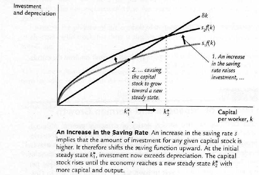
How Saving Affects Growth
The Solow
model shows that the saving rate is a key d
stock.
If the saving rate is high, the economy will have a large capital stock and a high level
of output in the steady state. If the saving rate is low, the economy will have a small capital
stock and a low level
discussions of fiscal policy, a government budget deficit can reduce national saving and crowd
out investment. Now that we can see that the long
are a lower capital stock and lower national income. This is why many economists are critical of
persistent budget deficits (G + TR > T)
FIGURE 11-5
What does the Solow model says about the relationship between saving and economic growth?
Higher s
aving leads to faster growth in the Solow model, but only temporary. An increase in
the
rate of saving raises growth only until the economy reaches a new steady state.
economy maintains a high saving rate, it will maintain a large capital stock
output, but it will not maintain a high rate of growth forever. Policies that alter the steady
state growth rate of income per person are said to have a growth effect. By contrast, a higher
saving rate is said to have a level effect,
growth rate —
is influenced by the saving rate in the steady state.
Saving and Investment Around the World
Why are some countries so rich while others are mired in poverty?
According to the Solow model, if a nation devotes a large fraction of its income to saving and
investment, it will have a high steady
saves and invests only a small fraction of its income, its s
low.
Learning Module on Macroeconomics
How Saving Affects Growth
model shows that the saving rate is a key d
eterminant of the steady
If the saving rate is high, the economy will have a large capital stock and a high level
of output in the steady state. If the saving rate is low, the economy will have a small capital
stock and a low level
of output in the steady state.
This conclusion sheds light on many
discussions of fiscal policy, a government budget deficit can reduce national saving and crowd
out investment. Now that we can see that the long
–
run consequences of a reduced saving rate
are a lower capital stock and lower national income. This is why many economists are critical of
persistent budget deficits (G + TR > T)
What does the Solow model says about the relationship between saving and economic growth?
aving leads to faster growth in the Solow model, but only temporary. An increase in
rate of saving raises growth only until the economy reaches a new steady state.
economy maintains a high saving rate, it will maintain a large capital stock
output, but it will not maintain a high rate of growth forever. Policies that alter the steady
state growth rate of income per person are said to have a growth effect. By contrast, a higher
saving rate is said to have a level effect,
because only the level of income per person
is influenced by the saving rate in the steady state.
Saving and Investment Around the World
Why are some countries so rich while others are mired in poverty?
According to the Solow model, if a nation devotes a large fraction of its income to saving and
investment, it will have a high steady
–
state capital stock and a high level of income. If a nation
saves and invests only a small fraction of its income, its s
teady state capital and income will be
Page | 6
eterminant of the steady
-state capital
If the saving rate is high, the economy will have a large capital stock and a high level
of output in the steady state. If the saving rate is low, the economy will have a small capital
This conclusion sheds light on many
discussions of fiscal policy, a government budget deficit can reduce national saving and crowd
run consequences of a reduced saving rate
are a lower capital stock and lower national income. This is why many economists are critical of
What does the Solow model says about the relationship between saving and economic growth?
aving leads to faster growth in the Solow model, but only temporary. An increase in
rate of saving raises growth only until the economy reaches a new steady state.
If the
economy maintains a high saving rate, it will maintain a large capital stock
and a high level of
output, but it will not maintain a high rate of growth forever. Policies that alter the steady
–
state growth rate of income per person are said to have a growth effect. By contrast, a higher
because only the level of income per person
– not its
is influenced by the saving rate in the steady state.
Why are some countries so rich while others are mired in poverty?
According to the Solow model, if a nation devotes a large fraction of its income to saving and
state capital stock and a high level of income. If a nation
teady state capital and income will be
Empirical evidence shows that high investment is associated with high income per person, as
the Solow Model predicts. The case of South Korea and Japan. The correlation between these
two variables is 0.25. Solo model’s prediction that the investment rate is a key determinant of
whether a country is rich or poor.
Why do rates of saving and investment vary so much from country to country? The reasons are
due to differences in tax policy, retirement patterns, development of financial markets, cultural
differences, political stability and political institutions.
Summary
• The Solow growth model shows that in the long run, an economy’s rate of savings
determines the size of its capital stock and thus its level of production
• The higher the rate of saving, the higher the stock of capital and the higher the level of
output
• In the Solow model, an increase in the rate of saving has a level effect on income per
person: it causes a period of rapid growth, but eventually that growth slows as the new
steady state is reached
• Thus, although a high saving rate yields a high steady-state level of output, saving by
itself can not generate persistent economic growth.
B. THE GOLDEN RULE LEVEL OF CAPITAL