Hindawi Publishing Corporation
Mathematical Problems in Engineering
Volume 2011, Article ID 810324, 18 pages
doi:10.1155/2011/810324
Research Article
Solution of Higher-Order ODEs Using Backward
Difference Method
Mohamed Bin Suleiman, Zarina Bibi Binti Ibrahim,
and Ahmad Fadly Nurullah Bin Rasedee
Department of Mathematics, Faculty of Science, UPM, Selangor Darul Ehsan, 43400 Serdang, Malaysia
Correspondence should be addressed to Mohamed Bin Suleiman, mohamed@math.upm.edu.my
Received 9 November 2010; Revised 25 March 2011; Accepted 13 May 2011
Academic Editor: Francesco Pellicano
Copyright q2011 Mohamed Bin Suleiman et al. This is an open access article distributed under
the Creative Commons Attribution License, which permits unrestricted use, distribution, and
reproduction in any medium, provided the original work is properly cited.
The current numerical technique for solving a system of higher-order ordinary differential equa-
tions ODEsis to reduce it to a system of first-order equations then solving it using first-order
ODE methods. Here, we propose a method to solve higher-order ODEs directly. The formulae
will be derived in terms of backward difference in a constant stepsize formulation. The method
developed will be validated by solving some higher-order ODEs directly with constant stepsize.
To simplify the evaluations of the integration coefficients, we find the relationship between various
orders. The result presented confirmed our hypothesis.
1. Introduction
Differential equations constantly arise in various branches of science and engineering. Many
of these problems are in the form of higher-order ordinary differential equations ODEs.
A few examples where these problems can be found are, in the motion of projectiles, the
bending of a thin clamped beam and population growth.
The popular practice for solving a system of higher-order ODEs is by reducing it to
a system of first-order equations and then solving with first-order methods. These methods
worked, so that methods for solving higher-order ODEs have been disregarded as robust
codes. However, the work by Krogh 1, Suleiman 2, Majid and Suleiman 3, and Omar
and Suleiman 4has revived the interest in solving higher-order ODEs directly and the
theoretical development of the methods.
Related works for solving higher-order ODEs can be found in Collatz 5,Gear6,
Krogh 1,7, and Suleiman 2. Krogh 7proposed the direct integration DImethod for
nonstiffproblems using modified divided difference while Suleiman 2proposed the DI

2 Mathematical Problems in Engineering
method using the standard divided difference. In this paper, we will derive the constant
stepsize backward difference formulae of solving higher-order ODEs up to third order. The
main reason for developing the constant stepsize formulae is that, in developing the theory
on convergence and stability, the approach is through constant stepsize formulation. Another
reason is that it is possible to use this formula in conjunction with other similar formulae as
in Majid and Suleiman 3to develop a code for variable stepsize and order.
The advantage of such a code is that the integration or differentiation constants are
calculated only once at the start of the first step of integration, whereas other formulations
calculate the constants at every step.
In this paper, we will focus only on nonstiffODEs of the form
ydfx,
Y,1.1
Yxfx, y, y,y
,…,y
d−1,
ηη, η,η
,…,η
d−1,
1.2
where
Yaηin the interval a≤x≤band dis the order of the ODE.
Without loss of generality, we will be considering the scalar equation in 1.1.
This paper will be organized as follows. First, the integration coefficients of the explicit
constant stepsize backward difference formulation of the DI method will be derived. Then,
the coefficients of the implicit method are formulated and their relationship with the explicit
coefficients is shown. We start the derivation with the coefficients of the first-order system,
which is given in Henrici 8. Next, the second-order coefficients are derived and their
relationship with the corresponding first-order coefficients is given, likewise the relationship
of the coefficients for the second- and third-order systems. Finally, the method developed
using backward difference will be validated numerically.
2. The Formulation of the Predict-Evaluate-Correct-Evaluate
(PECE) Multistep Method in Its Backward Difference Form
(MSBD) for Nonstiff Higher-Order ODEs
The code developed will be using the PECE mode. The predictor and corrector will have the
following form:
predictor:
pryd−t
n1
t−1
i0
hi
i!yd−t1
nhdk−1
i0
γd−t,i∇ifn,t1,2,…,d, 2.1
corrector:
yd−t
n1
t−1
i0
hi
i!yd−t1
nhdk−1
i0
γ∗
d−t,i∇ifn1,t1,2,…,d. 2.2

Mathematical Problems in Engineering 3
The corrector will be reformulated, so that it will be in terms of the predictor. The reformu-
lated corrector can be written as
yd−t
n1pryd−t
n1γd−t,k∇kprfn1,t1,2,…,d, 2.3
where prfn1indicates fn1evaluated using predicted values. The integration coefficient γd−t,i
and γ∗
d−t,i will be derived using the method of generating function. Finally, the constant
stepsize algorithm will be constructed and validated with some test problems and examples
from physical situations.
3. Derivation up to Third-Order Explicit Integration Coefficients
Integrating 1.1once yields
yxn1yxnxn1
xn
fx, y, y,y
dx. 3.1
Let Pnxbe the interpolating polynomial which interpolates the kvalues xn,f
n,
xn−1,f
n−1,…,xn−k1,f
n−k1, then
Pnx
k−1
i0
−1i−s
i∇ifn.3.2
Next, approximating fin 3.1with Pnxand letting
xxnsh or sx−xn
h3.3
gives us
yxn1yxn1
0
k−1
i0
−1i−s
i∇ifnds, 3.4
or
yxn1yxnh
k−1
i0
γ1,i∇ifn,3.5
where
γ1,i −1i1
0⎛
⎝−s
i⎞
⎠ds. 3.6

4 Mathematical Problems in Engineering
The generating function G1tfor the coefficients γ1,i is defined as follows:
G1t
∞
i0
γ1,iti.3.7
Substituting γ1,i in 3.6in G1tgives
G1t
∞
i0
−ti1
0−s
ids,
G1t1
0
1−t−sds,
G1t1
0
e−slog1−tds
3.8
which leads to
G1t−1−t−1
log1−t−1
log1−t.3.9
Equation 3.9can be written as
−∞
i0
γ1,itilog1−tt
1−t3.10
or
γ1,0γ1,1tγ1,2t2γ1,3t3···tt2
2t3
3t4
4···t1tt2t3···.3.11
Hence, the coefficients of γ1,k are given by
k
i0γ1,i
k−i11,
γ1,k 1−
k−1
i0γ1,i
k−i1k1,2,…, γ
1,01.
3.12
Mathematical Problems in Engineering 5
4. Second-Order ODE Formulae
Integrate 1.1twice for second-order ODEs where d2. Integrating once leads to the same
coefficients as given in 3.6. Integrating twice yields
yxn1yxnhyxnh2k
i0
γ2,i∇ifn.4.1
Substituting xwith sgives
γ2,i −1i1
0
1−s
1! −s
ids. 4.2
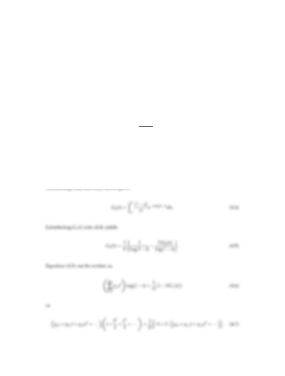
The generating function G2tof the coefficients γ2,i is defined as follows
G2t
∞
i0
γ2,iti.4.3