Solution Manual Chapter 9 Differential Analysis Of

PROPRIETARY AND CONFIDENTIAL

This Manual is the proprietary property of The McGraw-Hill

Companies, Inc. (“McGraw-Hill”) and protected by copyright and other

state and federal laws. By opening and using this Manual the user

agrees to the following restrictions, and if the recipient does not agree

to these restrictions, the Manual should be promptly returned unopened

to McGraw-Hill: This Manual is being provided only to authorized

professors and instructors for use in preparing for the classes using

the affiliated textbook. No other use or distribution of this Manual

is permitted. This Manual may not be sold and may not be

distributed to or used by any student or other third party. No part

of this Manual may be reproduced, displayed or distributed in any

form or by any means, electronic or otherwise, without the prior

written permission of McGraw-Hill.

Solution Manual, Chapter 9 – Differential Analysis of Fluid Flow

Chapter 9

Differential

Analysis

General and Mathematical Problems

9-1C

Solution We are to explain the fundamental differences between a flow domain

and a control volume.

Analysis A control volume is used in an integral, control volume solution. It

is a volume over which all mass flow rates, forces, etc. are specified over the entire

control surface of the control volume. In a control volume analysis we do not know or

care about details inside the control volume. Rather, we solve for gross features of the

flow such as net force acting on a body. A flow domain, on the other hand, is also a

volume, but is used in a differential analysis. Differential equations of motion are

solved everywhere inside the flow domain, and we are interested in all the details

inside the flow domain.

Discussion Note that we also need to specify what is happening at the boundaries

of a flow domain – these are called boundary conditions.

9-2C

Solution We are to explain what we mean by coupled differential equations.

Analysis A set of coupled differential equations simply means that the

equations are dependent on each other and must be solved together rather than

separately. For example, the equations of motion for fluid flow involve velocity

variables in both the conservation of mass equation and the momentum equation. To

solve for these variables, we must solve the coupled set of differential equations

together.

Discussion In some very simple fluid flow problems, the equations become

uncoupled, and are easier to solve.

9-1

Solution Manual, Chapter 9 – Differential Analysis of Fluid Flow

9-3C

Solution We are to discuss the number of unknowns and the equations needed

to solve for those unknowns for a three-dimensional, unsteady, incompressible flow

field.

Analysis There are four unknowns (velocity components u, v, w, and pressure

P) and thus we need to solve four equations:

− one from conservation of mass which is a scalar equation

− three from Newton’s second law which is a vector equation

Discussion These equations are also coupled in general.

9-4C

Solution We are to discuss the number of unknowns and the equations needed

to solve for those unknowns for a three-dimensional, unsteady, compressible flow

field with significant variations in both temperature and density.

Analysis There are six unknowns (velocity components u, v, w,

ρ

, T, and P)

and thus we need to solve six equations:

− one from conservation of mass which is a scalar equation

− three from Newton’s second law which is a vector equation

− one from the energy equation which is a scalar equation

− one from an equation of state (e.g. ideal gas law) which is a scalar equation

Discussion These equations are also coupled in general.

9-5C

Solution We are to express the divergence theorem in words.

Analysis For vector

G

, the volume integral of the divergence of G

G

over

volume V is equal to the surface integral of the normal component of G

G

taken

over the surface A that encloses the volume.

Discussion The divergence theorem is also called Gauss’s theorem.

9-2

Solution Manual, Chapter 9 – Differential Analysis of Fluid Flow

9-6

Solution We are to transform a position from Cartesian to cylindrical

coordinates.

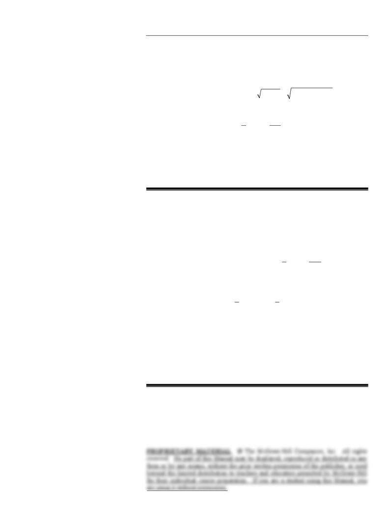
Analysis We use the coordinate transformations provided in this chapter,

()()

22

22 4 m 3 m 5 mrxy=+= + = (1)

and

11 o

3 m

tan tan 36.87 0.6435 radians

4 m

y

x

θ

−−



== ==



 (2)

Coordinate z remains unchanged. Thus,

Position in cylindrical coordinates:

(

)( )

,,xrz

θ

==5 m, 0.6435 radians, – 4 m

G

(3)

Discussion Notice that the units of

θ

are radians since angles are dimensionless.

9-7

Solution We are to calculate a truncated Taylor series expansion for a given

function and compare our result with the exact value.

Analysis The algebra here is simple since d(ex)/dx = ex. The Taylor series

expansion is

Taylor series expansion: 00 0 0

23

0

11

() 232

xx x x

f x dx e e dx e dx e dx ...

+

=+ + + +

× (1)

We plug x0 = 0 and dx = –0.1 into Eq. 1,

Truncated Taylor series expansion:

23

11

( 0.1) 1 1 ( 0.1) 1 ( 0.1) 1 ( 0.1) 0.9048333…

26

f−≈+×−+××− +××− = (2)

We compare Eq. 2 with the exact value,

Exact value:

0.1

( 0.1) 0.904837418…fe

−

−= = (3)

Comparing Eqs. 2 and 3 we see that our approximation is good to four or five

significant digits.

Discussion The smaller the value of dx, the better the approximation. You can

easily convince yourself of this by trying dx = 0.01 instead.

9-3

Solution Manual, Chapter 9 – Differential Analysis of Fluid Flow

9-8

Solution We are to calculate the divergence of a given vector.

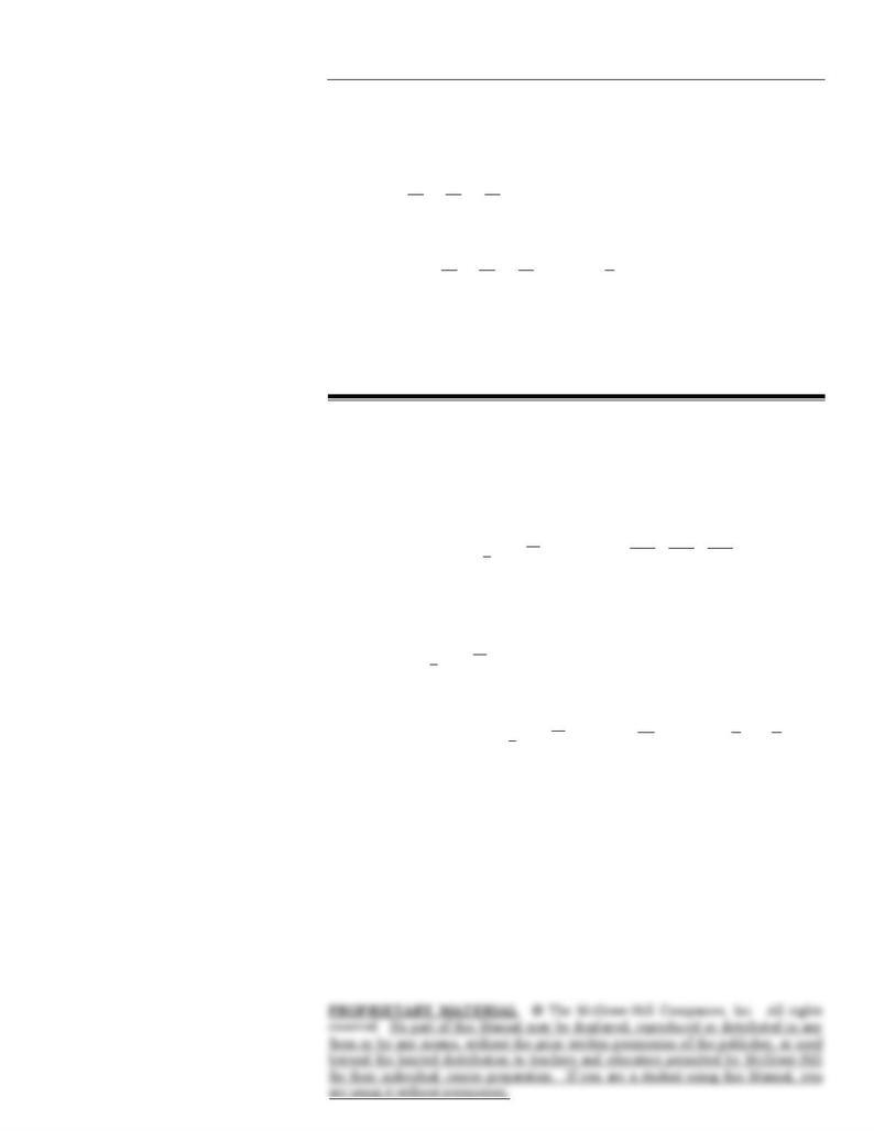
Analysis We calculate the divergence of G

G

by taking the dot product of the del

operator ijk

x

yz

∂

∂∂

+ +∇=

∂

∂∂

G

G with G

G

,

Divergence of G

G

:

22

1

22

2

Gijkxzixjzkz z

xy z



∂∂∂



02

∇

⋅= + + ⋅ − + = +− =



∂∂∂

 0

G

GGG

G

It turns out that for this special case, the divergence of G is zero.

Discussion If G

G

were a velocity vector, this would mean that the flow field is

incompressible.

9-9

Solution We are to perform both integrals of the divergence theorem for a

given vector and volume, and verify that they are equal.

Analysis We do the volume integral first:

Volume integral:

()

111

000

111

000

4 2

xyz y

xz

Vxyz

xyz

G

GG

GdV dzdydx

xyz

zyydzdydx

===

∂



∂∂

∇⋅ = + +



∂∂∂



=−+

∫∫∫∫

∫∫∫

G

(1)

The term in parentheses in Eq. 1 reduces to (4z – y), and we integrate this over z first,

()

11 11

1

2

0

00 00

22

xy xy

z

Vxy xy

GdV z yz dydx y dydx

== ==

=

== ==



∇⋅ = − = −



∫∫∫ ∫∫

G

Then we integrate over y and then over x,

Volume integral:

1

2

11

00

0

3

222

y

xx

Vx x

y

GdV y dx dx

=

==

=



∇

⋅= − = =





∫∫ ∫

3

2

G

G (2)

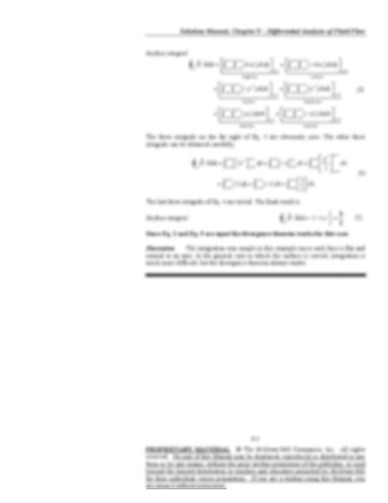
Next we calculate the surface integral of the divergence theorem. There are

six faces of the cube, and unit vector n

G

points outward from each surface. Thus we

split the area integral into six parts and sum them. For example, the right-most face

has n

G

= (1,0,0), so Gn

⋅

G

= 4xz on this face. The bottom face has n

G

= (0,–1,0), so

G = y2 on this face. The surface integral is then G⋅n

G

9-4