PROPRIETARY AND CONFIDENTIAL
This Manual is the proprietary property of The McGraw-Hill
Companies, Inc. (“McGraw-Hill”) and protected by copyright and other
state and federal laws. By opening and using this Manual the user
agrees to the following restrictions, and if the recipient does not agree
to these restrictions, the Manual should be promptly returned unopened
to McGraw-Hill: This Manual is being provided only to authorized
professors and instructors for use in preparing for the classes using
the affiliated textbook. No other use or distribution of this Manual
is permitted. This Manual may not be sold and may not be
distributed to or used by any student or other third party. No part
of this Manual may be reproduced, displayed or distributed in any
form or by any means, electronic or otherwise, without the prior
written permission of McGraw-Hill.

Solution Manual, Chapter 15 – Computational Fluid Dynamics
Chapter 15 –
Computational
Fluid Dynamics
Fundamentals, Grid Generation, and Boundary Conditions
15-1C
Solution We are to list the unknowns and the equations for a given flow
situation.
Analysis There are only three unknowns in this problem, u, v, and P (orP′).
Thus, we require three equations: continuity, x momentum (or x component of
Navier-Stokes), and y momentum (or y component of Navier-Stokes). These
equations, when combined with the appropriate boundary conditions, are sufficient to
solve the problem.
Discussion The actual equations to be solved by the computer are discretized
versions of the differential equations.
15-2C
Analysis
(a) A computational domain is a region in space (either 2-D or 3-D) in which the
numerical equations of fluid flow are solved by CFD. The computational
domain is bounded by edges (2-D) or faces (3-D) on which boundary conditions
are applied.
(b) A mesh is generated by dividing the computational domain into tiny cells.
The numerical equations are then solved in each cell of the mesh. A mesh is also
called a grid.
(c) A transport equation is a differential equation representing how some
property is transported through a flow field. The transport equations of fluid
mechanics are conservation equations. For example, the continuity equation is a
differential equation representing the transport of mass, and also conservation of
mass. The Navier-Stokes equation is a differential equation representing the
transport of linear momentum, and also conservation of linear momentum.
(d) Equations are said to be coupled when at least one of the variables
(unknowns) appears in more than one equation. In other words, the equations
cannot be solved alone, but must be solved simultaneously with each other. This
is the case with fluid mechanics since each component of velocity, for example,
appears in the continuity equation and in all three components of the Navier-
Stokes equation.
15-1
Solution Manual, Chapter 15 – Computational Fluid Dynamics
15-3C
Solution We are to discuss the difference between nodes and intervals and
analyze a given computational domain in terms of nodes and intervals.
Analysis Nodes are points along an edge of a computational domain that
represent the vertices of cells. In other words, they are the points where corners of
the cells meet. Intervals, on the other hand, are short line segments between
nodes. Intervals represent the small edges of cells themselves. In Fig. P15-3 there are
6 nodes and 5 intervals on the top and bottom edges. There are 5 nodes and 4
intervals on the left and right edges.
Discussion We can extend the node and interval concept to three dimensions.
15-4C
Solution For a given computational domain with specified nodes and intervals
we are to compare a structured grid and an unstructured grid and discuss.
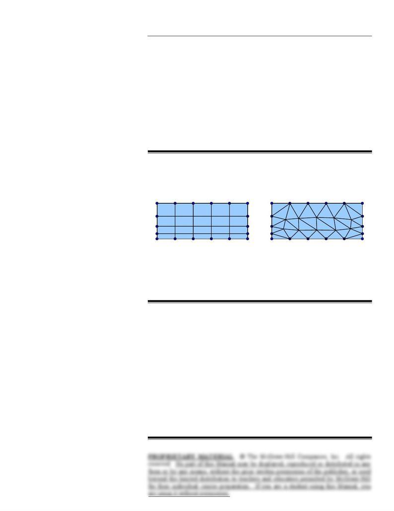
Analysis We construct the two grids in Fig. 1.
(a) (b)
FIGURE 1
A structured (a) and unstructured (b) grid
generated for a given node distribution on
the edges of the computational domain of
Fig. P15-3.
There are 5 × 4 = 20 cells in the structured grid, and there are 36 cells in the
unstructured grid.
Discussion Depending on how individual students construct their unstructured
grid, the shape, size, and number of cells may differ considerably.
15-5C
Solution We are to summarize the eight steps involved in a typical CFD
analysis.
Analysis We list the steps in the order presented in this chapter:
1. Specify a computational domain and generate a grid.
2. Specify boundary conditions on all edges or faces.
3. Specify the type of fluid and its properties.
4. Specify numerical parameters and solution algorithms.
5. Apply initial conditions as a starting point for the iteration.
6. Iterate towards a solution.
7. After convergence, analyze the results (post processing).
8. Calculate global and integral properties as needed.
Discussion The order of some of the steps is interchangeable, particularly Steps 2
through 5.
15-2

Solution Manual, Chapter 15 – Computational Fluid Dynamics
15-6C
Solution We are to explain why the cylinder should not be centered
horizontally in the computational domain.
Analysis Flow separates over bluff bodies, generating a wake with reverse
flow and eddies downstream of the body. There are no such problems upstream.
Hence it is always wise to extend the downstream portion of the domain as far as
necessary to avoid reverse flow problems at the outlet boundary.
Discussion The same problems arise at the outlet of ducts and pipes – sometimes
we need to extend the duct to avoid reverse flow at the outlet boundary.
15-7C
Analysis
(a) In a CFD solution, we typically iterate towards a solution. In order to get
started, we make some initial conditions for all the variables (unknowns) in
the problem. These initial conditions are wrong, of course, but they are
necessary as a starting point. Then we begin the iteration process, eventually
obtaining the solution.
(b) A residual is a measure of how much our variables differ from the “exact”
solution. We construct a residual by putting all the terms of a transport equation
on one side, so that the terms all add to zero if the solution is correct. As we
iterate, the terms will not add up to zero, and the remainder is called the residual.
As the CFD solution iterates further, the residual should (hopefully) decrease.
(c) Iteration is the numerical process of marching towards a final solution,
beginning with initial conditions, and progressively correcting the solution. As
the iteration proceeds, the variables converge to their final solution as the
residuals decrease.
(d) Once the CFD solution has converged, post processing is performed on the
solution. Examples include plotting velocity and pressure fields, calculating
global properties, generating other flow quantities like vorticity, etc. Post
processing is performed after the CFD solution has been found, and does not
change the results. Post processing is generally not as CPU intensive as the
iterative process itself.
15-8C
Analysis
(a) With multigridding, solutions of the equations of motion are obtained on a
coarse grid first, followed by successively finer grids. This speeds up
convergence because the gross features of the flow are quickly established on the
coarse grid, and then the iteration process on the finer grid requires less time.
(b) In some CFD codes, a steady flow is treated as though it were an unsteady
flow. Then, an artificial time is used to march the solution in time. Since the
solution is steady, however, the solution approaches the steady-state solution as
“time” marches on. In some cases, this technique yields faster convergence.
15-3
Solution Manual, Chapter 15 – Computational Fluid Dynamics
15-9C
Solution We are to list the boundary conditions that are applicable to a given
edge, and we are to explain why other boundary conditions are not applicable.
Analysis We may apply the following boundary conditions: outflow, pressure
inlet, pressure outlet, symmetry (to be discussed), velocity inlet, and wall. The
curved edge cannot be an axis because an axis must be a straight line. The edge
cannot be a fan or interior because such edges cannot be at the outer boundary of a
computational domain. Finally, the edge cannot be periodic since there is no other
edge along the boundary of the computational domain that is of identical shape
(a periodic boundary must have a “partner”). The symmetry boundary condition
merits further discussion. Numerically, gradients of flow variables in the direction
normal to a symmetry boundary condition are set to zero, and there is no
mathematical reason why the curved right edge of the present computational domain
cannot be set as symmetry. However, you would be hard pressed to think of a
physical situation in which a curved edge like that of Fig. P15-9 would be a valid
symmetry boundary condition.
Discussion Just because you can set a boundary condition and generate a CFD
result does not guarantee that the result is physically meaningful.
15-10C
Solution We are to discuss the standard method to test for adequate grid
resolution.
Analysis The standard method to test for adequate grid resolution is to increase
the resolution (by a factor of 2 in all directions if feasible) and repeat the
simulation. If the results do not change appreciably, the original grid is deemed
adequate. If, on the other hand, there are significant differences between the two
solutions, the original grid is likely of inadequate resolution. In such a case, an even
finer grid should be tried until the grid is adequately resolved.
Discussion Keep in mind that if the boundary conditions are not specified
properly, or if the chosen turbulence model is not appropriate for the flow being
simulated by CFD, no amount of grid refinement is going to make the solution more
physically correct.
15-4