© The McGraw-Hill Companies, Inc., 2012. All rights reserved.
Solutions Manual, Chapter 5 193
Chapter 5
Cost-Volume-Profit Relationships
Solutions to Questions
5-1 The contribution margin (CM) ratio is
the ratio of the total contribution margin to total
sales revenue. It is used in target profit and
break-even analysis and can be used to quickly
estimate the effect on profits of a change in
sales revenue.
5-2 Incremental analysis focuses on the
changes in revenues and costs that will result
from a particular action.
5-3 All other things equal, Company B, with
its higher fixed costs and lower variable costs,
will have a higher contribution margin ratio than
Company A. Therefore, it will tend to realize a
larger increase in contribution margin and in
profits when sales increase.
5-4 Operating leverage measures the impact
on net operating income of a given percentage
change in sales. The degree of operating
leverage at a given level of sales is computed by
dividing the contribution margin at that level of
sales by the net operating income at that level
of sales.
5-5 The break-even point is the level of
sales at which profits are zero.
5-6 (a) If the selling price decreased, then
the total revenue line would rise less steeply,
and the break-even point would occur at a
higher unit volume. (b) If the fixed cost
increased, then both the fixed cost line and the
total cost line would shift upward and the break–
even point would occur at a higher unit volume.
(c) If the variable cost increased, then the total
cost line would rise more steeply and the break–
even point would occur at a higher unit volume.
5-7 The margin of safety is the excess of
budgeted (or actual) sales over the break-even
volume of sales. It is the amount by which sales
can drop before losses begin to be incurred.
5-8 The sales mix is the relative proportions
in which a company’s products are sold. The
usual assumption in cost-volume-profit analysis
is that the sales mix will not change.
5-9 A higher break-even point and a lower
net operating income could result if the sales
mix shifted from high contribution margin
products to low contribution margin products.
Such a shift would cause the average
contribution margin ratio in the company to
decline, resulting in less total contribution
margin for a given amount of sales. Thus, net
operating income would decline. With a lower
contribution margin ratio, the break-even point
would be higher because more sales would be
required to cover the same amount of fixed
costs.

© The McGraw-Hill Companies, Inc., 2012. All rights reserved.
194 Managerial Accounting, 14th Edition
Exercise 5-1 (20 minutes)
1. The new income statement would be:
Total
Per Unit
Sales (8,050 units) …..
$209,300
$26.00
Variable expenses ……
144,900
18.00
Contribution margin ….
64,400
$ 8.00
Fixed expenses ……….
56,000
Net operating income .
$ 8,400
You can get the same net operating income using the following
approach.
Original net operating income ..
$8,000
Change in contribution margin
(50 units × $8.00 per unit) ….
400
New net operating income …….
$8,400
2. The new income statement would be:
Total
Per Unit
Sales (7,950 units) …………
$206,700
$26.00
Variable expenses ………….
143,100
18.00
Contribution margin ………..
63,600
$ 8.00
Fixed expenses ……………..
56,000
Net operating income ……..
$ 7,600
You can get the same net operating income using the following
approach.
Original net operating income ………….
$8,000
Change in contribution margin
(-50 units × $8.00 per unit) ………….
(400)
New net operating income ………………
$7,600

© The McGraw-Hill Companies, Inc., 2012. All rights reserved.
Solutions Manual, Chapter 5 195
Exercise 5-1 (continued)
3. The new income statement would be:
Total
Per Unit
Sales (7,000 units) …….
$182,000
$26.00
Variable expenses ……..
126,000
18.00
Contribution margin ……
56,000
$ 8.00
Fixed expenses …………
56,000
Net operating income …
$ 0
Note: This is the company‘s break-even point.

© The McGraw-Hill Companies, Inc., 2012. All rights reserved.
196 Managerial Accounting, 14th Edition
Exercise 5-2 (30 minutes)
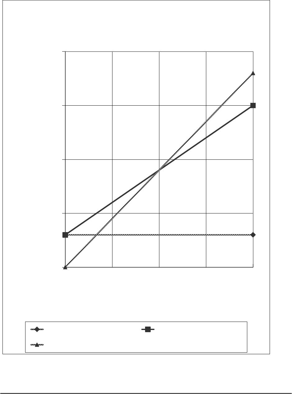
1. The CVP graph can be plotted using the three steps outlined in the text.
The graph appears on the next page.
Step 1. Draw a line parallel to the volume axis to represent the total
fixed expense. For this company, the total fixed expense is $12,000.
Step 2. Choose some volume of sales and plot the point representing
total expenses (fixed and variable) at the activity level you have
selected. We’ll use the sales level of 2,000 units.
Fixed expenses ……………………………………………
$12,000
Variable expenses (2,000 units × $24 per unit) …..
48,000
Total expense ……………………………………………..
$60,000
Step 3. Choose some volume of sales and plot the point representing
total sales dollars at the activity level you have selected. We’ll use the
sales level of 2,000 units again.
Total sales revenue (2,000 units × $36 per unit) …
$72,000
2. The break-even point is the point where the total sales revenue and the
total expense lines intersect. This occurs at sales of 1,000 units. This
can be verified as follows:
Profit
= Unit CM × Q – Fixed expenses
= ($36 − $24) × 1,000 − $12,000
= $12 × 1,000 − $12,000
= $12,000 − $12,000
= $0
© The McGraw-Hill Companies, Inc., 2012. All rights reserved.
Solutions Manual, Chapter 5 197
Exercise 5-2 (continued)
$0
$20,000
$40,000
$60,000
$80,000
0 500 1,000 1,500 2,000
Dollars
Volume in Units
CVP Graph
Fixed Expense Total Expense
Total Sales Revenue
© The McGraw-Hill Companies, Inc., 2012. All rights reserved.
198 Managerial Accounting, 14th Edition
Exercise 5-3 (15 minutes)
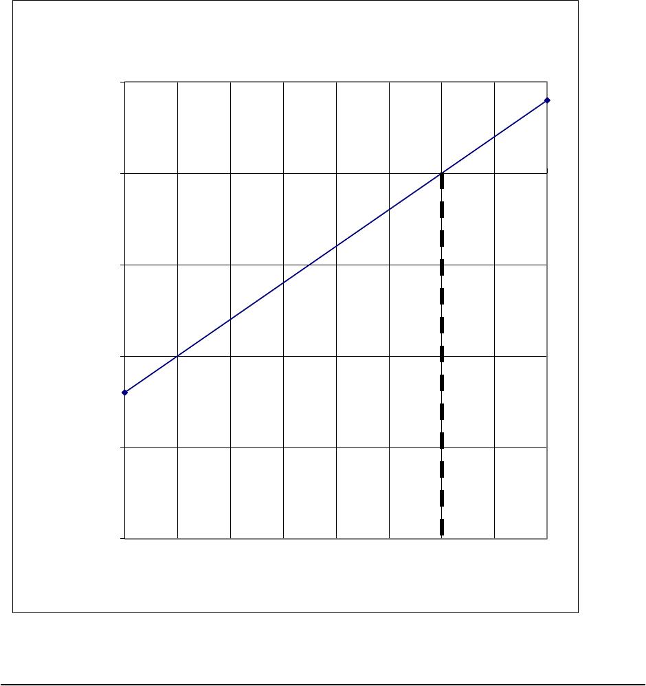
1. The profit graph is based on the following simple equation:
Profit
= Unit CM × Q − Fixed expenses
Profit
= ($19 − $15) × Q − $12,000
Profit
= $4 × Q − $12,000
To plot the graph, select two different levels of sales such as Q=0 and
Q=4,000. The profit at these two levels of sales are -$12,000 (= $4 × 0
− $12,000) and $4,000 (= $4 × 4,000 − $12,000).
-$20,000
-$15,000
-$10,000
-$5,000
$0
$5,000
0 500 1,000 1,500 2,000 2,500 3,000 3,500 4,000
Profit
Sales Volume in Units
Profit Graph

© The McGraw-Hill Companies, Inc., 2012. All rights reserved.
Solutions Manual, Chapter 5 199
Exercise 5-3 (continued)
2. Looking at the graph, the break-even point appears to be 3,000 units.
This can be verified as follows:
Profit
= Unit CM × Q − Fixed expenses
= $4 × Q − $12,000
= $4 × 3,000 − $12,000
= $12,000 − $12,000 = $0

© The McGraw-Hill Companies, Inc., 2012. All rights reserved.
200 Managerial Accounting, 14th Edition
Exercise 5-4 (10 minutes)
1. The company’s contribution margin (CM) ratio is:
Total sales ……………………….
$300,000
Total variable expenses ………
240,000
= Total contribution margin …
$ 60,000
÷ Total sales …………………….
$300,000
= CM ratio ……………………….
20%
2. The change in net operating income from an increase in total sales of
$1,500 can be estimated by using the CM ratio as follows:
Change in total sales ………………….
$1,500
× CM ratio ……………………………….
20%
= Estimated change in net
operating income …………………….
$ 300
This computation can be verified as follows:
Total sales ……………….
$300,000
÷ Total units sold ………
40,000
units
= Selling price per unit .
$7.50
per unit
Increase in total sales …
$1,500
÷ Selling price per unit .
$7.50
per unit
= Increase in unit sales
200
units
Original total unit sales .
40,000
units
New total unit sales ……
40,200
units
Original
New
Total unit sales………….
40,000
40,200
Sales ………………………
$300,000
$301,500
Variable expenses ……..
240,000
241,200
Contribution margin ……
60,000
60,300
Fixed expenses …………
45,000
45,000
Net operating income …
$ 15,000
$ 15,300

© The McGraw-Hill Companies, Inc., 2012. All rights reserved.
Solutions Manual, Chapter 5 201
Exercise 5-5 (20 minutes)
1. The following table shows the effect of the proposed change in monthly
advertising budget:
Sales With
Additional
Current
Advertising
Sales
Budget
Difference
Sales ………………………
$225,000
$240,000
$15,000
Variable expenses ……..
135,000
144,000
9,000
Contribution margin ……
90,000
96,000
6,000
Fixed expenses …………
75,000
83,000
8,000
Net operating income …
$ 15,000
$ 13,000
$(2,000)
Assuming that there are no other important factors to be considered,
the increase in the advertising budget should not be approved because
it would lead to a decrease in net operating income of $2,000.
Alternative Solution 1
Expected total contribution margin:
$240,000 × 40% CM ratio ………………
$96,000
Present total contribution margin:
$225,000 × 40% CM ratio ………………
90,000
Incremental contribution margin ………..
6,000
Change in fixed expenses:
Less incremental advertising expense .
8,000
Change in net operating income …………
$(2,000)
Alternative Solution 2
Incremental contribution margin:
$15,000 × 40% CM ratio ……………….
$6,000
Less incremental advertising expense ….
8,000
Change in net operating income …………
$(2,000)

© The McGraw-Hill Companies, Inc., 2012. All rights reserved.
202 Managerial Accounting, 14th Edition
Exercise 5-5 (continued)
2. The $3 increase in variable expenses will cause the unit contribution
margin to decrease from $30 to $27 with the following impact on net
operating income:
Expected total contribution margin with the
higher-quality components:
3,450 units × $27 per unit …………………………
$93,150
Present total contribution margin:
3,000 units × $30 per unit …………………………
90,000
Change in total contribution margin ………………..
$ 3,150
Assuming no change in fixed expenses and all other factors remain the
same, the higher-quality components should be used.

© The McGraw-Hill Companies, Inc., 2012. All rights reserved.
Solutions Manual, Chapter 5 203
Exercise 5-6 (10 minutes)
1. The equation method yields the required unit sales, Q, as follows:
Profit
= Unit CM × Q − Fixed expenses
$6,000
= ($140 − $60) × Q − $40,000
$6,000
= ($80) × Q − $40,000
$80 × Q
= $6,000 + $40,000
Q
= $46,000 ÷ $80
Q
= 575 units
2. The formula approach yields the required unit sales as follows:
Target profit + Fixed expenses
Units sold to attain =
the target profit Unit contribution margin
$8,000 + $40,000
= $80 per unit
$48,000
= $80 per unit
= 600 units
Exercise 5-7 (20 minutes)
1. The equation method yields the break-even point in unit sales, Q, as
follows:
Profit
= Unit CM × Q − Fixed expenses
$0
= ($8 − $6) × Q − $5,500
$0
= ($2) × Q − $5,500
$2Q
= $5,500
Q
= $5,500 ÷ $2
Q
= 2,750 baskets
2. The equation method can be used to compute the break-even point in
sales dollars as follows:
Unit contribution margin
CM ratio = Unit selling price
$2
= = 0.25
= 0.25 × Sales − $5,500
= $5,500
= $5,500 ÷ 0.25
= $22,000