SOLOW GROWTH MODEL
-The Solow Growth Model, for which Robert Solow of the
Massachusetts Institute of Technology received the Nobel Prize, is
probably the best known model of economic growth
– Although in some respects Solow’s Model describes a developed
economy better than a developing one, it remains a basic reference
point for the literature on growth and development
– It implies that economies will conditionally converge to the same level
of income if they have the same rates of savings, depreciation, labor
force growth, and productivity growth
– Thus the Solow Model is the basic framework for the study of
convergence across countries
– The key modification from the Harrod-Domar Growth Model, is that
the Solow Model allows for substitution between capital and labor. In
the process, it assumes that there are diminishing returns to the use of
these inputs

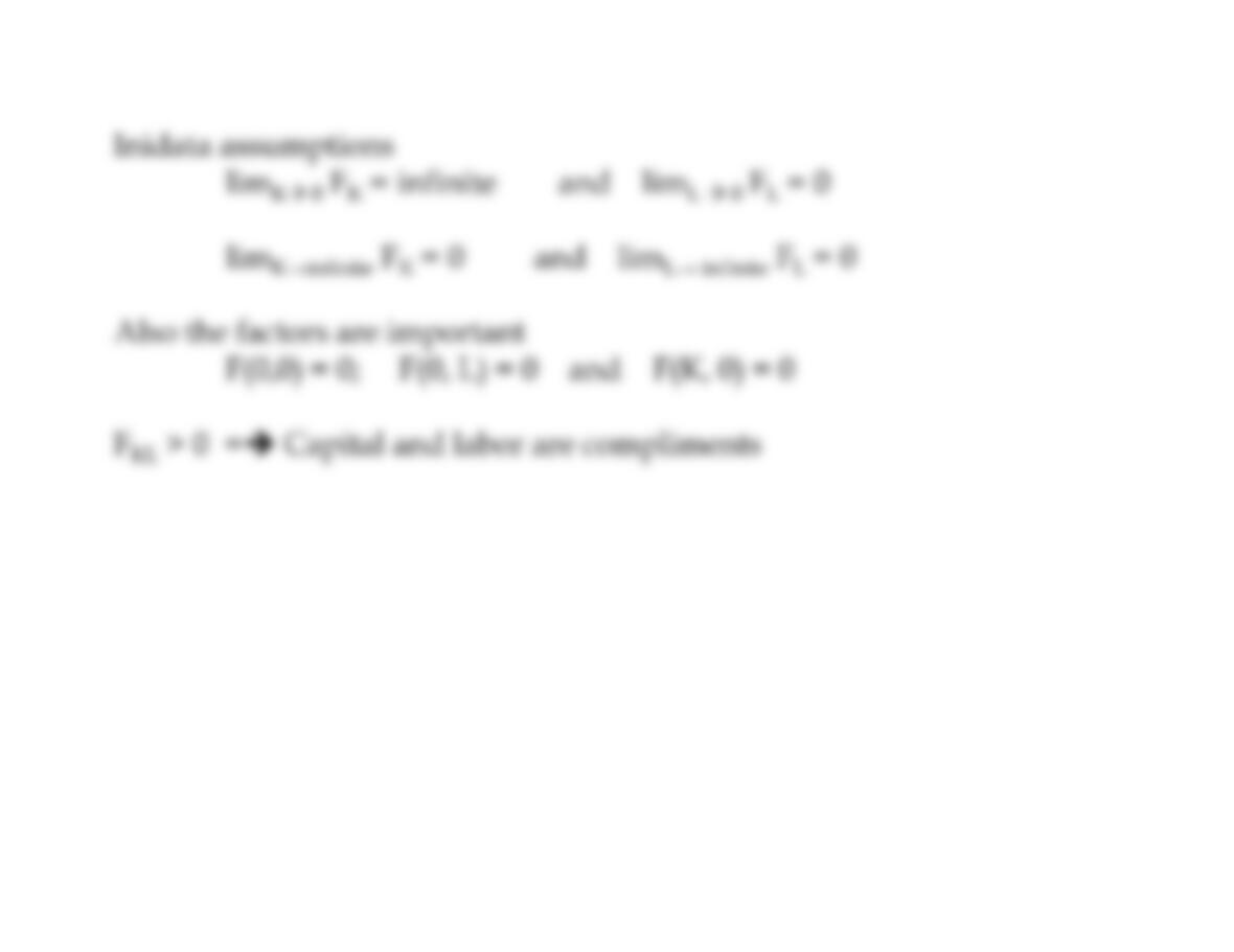
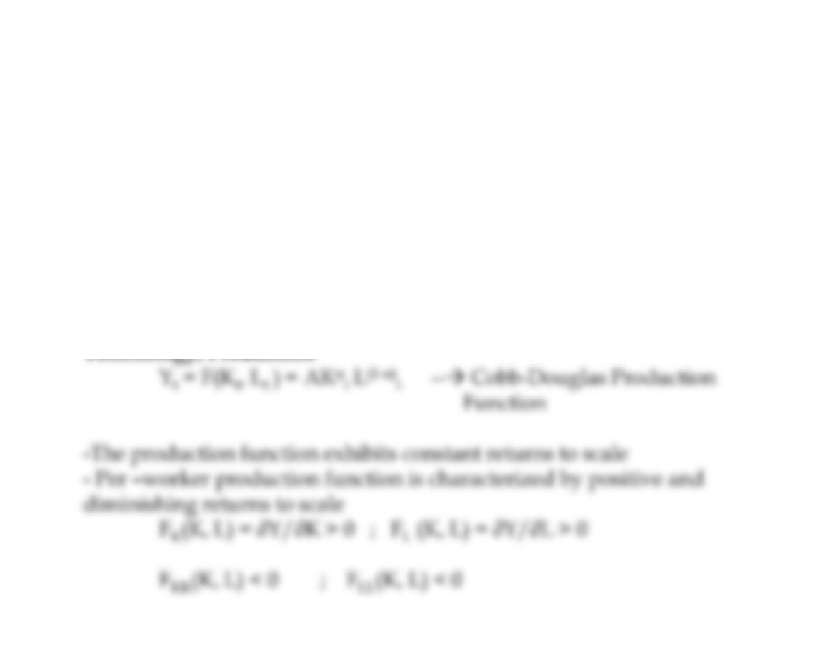
-The aggregate production function, Y = F(K,L) is assumed
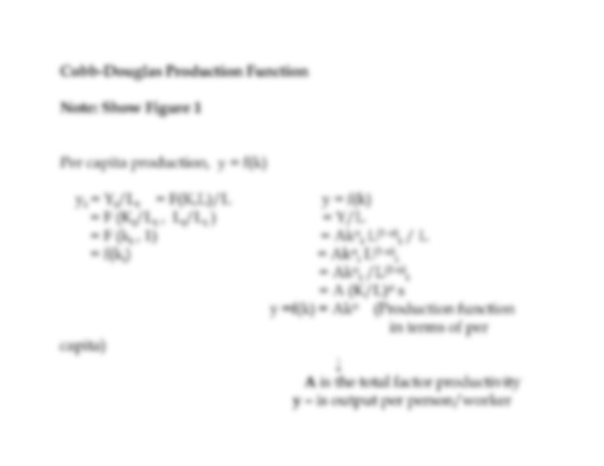
characterized by constant returns to scale. For example, in the special
case known as the Cobb-Douglas production function
Fast Overview of the Model
Assumptions:
-Time (dynamic model); Close economy
– Variables and parameters
– per capita or per worker
– goods market
– Technology, Production Function; Constant Returns to Scale, positive
but diminishing marginal returns
– Capital accumulation equation
– Converting variables into per-capita terms
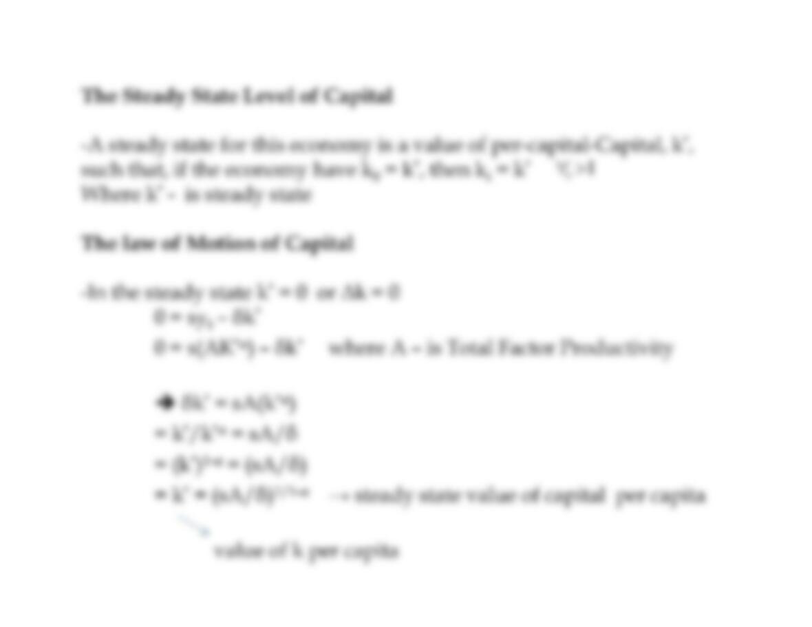
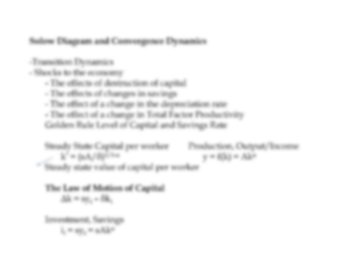
– The steady state
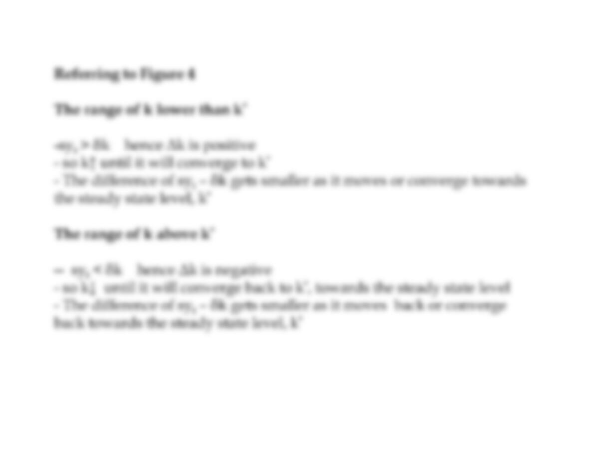
– Solow Diagram
– Transition dynamics, time series
-Shocks, effect of a change in savings, depreciation, Total factor
productivity, etc…

Variables endogenous, dynamic
Yt: output, income Lt: Labor, population, workers
Kt: capital It: Investment, savings
Ct: consumption
Where: Yt– Aggregate output; Kt– Aggregate capital
Lt– Aggregate labor; It– Aggregate investment
Ct– Aggregate consumption
Parameters: exogenous, constant
s : savings rate (between 0 and 1)
δ : depreciation rate (between 0 and 1)
g = gA: growth rate of technology
n = gL: population growth rate
Per capita variables
kt= Kt/Lt; yt= Yt/Lt;
it= It/Ltct= Ct/Lt

Goods Market
Yt= Ct+ It
It= sYt
Ct= (1 – s)Yt
Technology, Production
Yt= F(Kt, Lt) = AkαtL(1-α)t
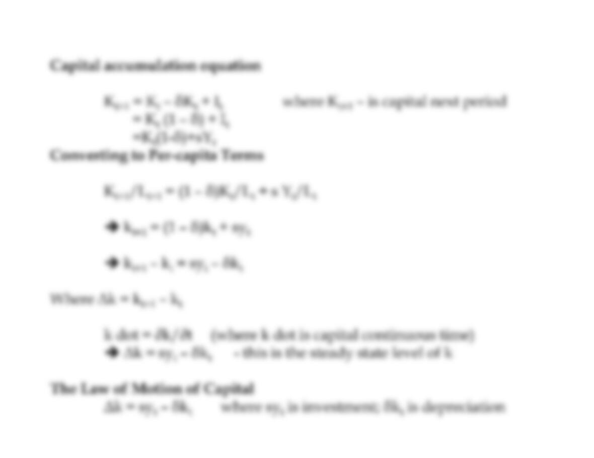
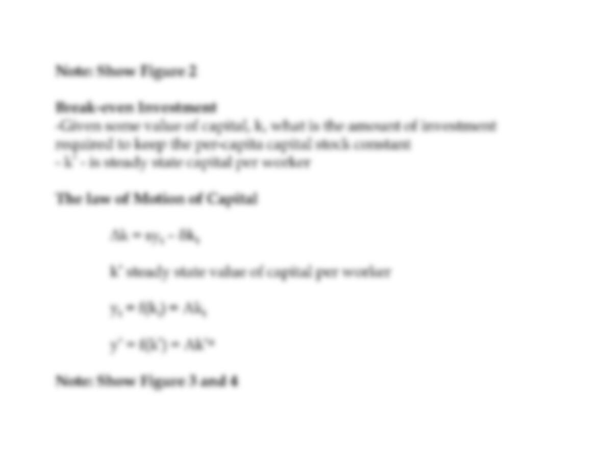
Law of Motion of Capital or Capital Accumulation Equation
Kt+1 = Kt– δKt+ It
–The Law of Motion of Capital – tells how the capital changes
through time
aka “Neoclassical Growth Model”
aka “Solow Swan Growth Model”
aka “Exogenous Growth Model”
Production Function: Yt= F(Kt, Lt)
Solow Model
-Shows that in the long run the economy’s rate of savings determines
the size of capital stock and therefore the level of production and its
per capita output
–The higher the level of savings –the higher the stock of capital
and the higher the level of output
– The model relates the economic growth the changes in factors like L
and K and interest rates, depreciation, growth and level of technology