10–1
CHAPTER 10
DETERMINING HOW COSTS BEHAVE
10–1 The two assumptions are
1. Variations in the level of a single activity (the cost driver) explain the variations in the
related total costs.
2. Cost behavior is approximated by a linear cost function within the relevant range. A
linear cost function is a cost function where, within the relevant range, the graph of total
costs versus the level of a single activity forms a straight line.
10–2 Three alternative linear cost functions are
1. Variable cost function––a cost function in which total costs change in proportion to the
changes in the level of activity in the relevant range.
2. Fixed cost function––a cost function in which total costs do not change with changes in
the level of activity in the relevant range.
3. Mixed cost function––a cost function that has both variable and fixed elements. Total
costs change but not in proportion to the changes in the level of activity in the relevant
range.
10–3 A linear cost function is a cost function where, within the relevant range, the graph of
total costs versus the level of a single activity related to that cost is a straight line. An example of
a linear cost function is a cost function for use of a videoconferencing line where the terms are a
fixed charge of $10,000 per year plus a $2 per minute charge for line use. A nonlinear cost
function is a cost function where, within the relevant range, the graph of total costs versus the
level of a single activity related to that cost is not a straight line. Examples include economies of
scale in advertising where an agency can double the number of advertisements for less than twice
the costs, step–cost functions, and learning–curve–based costs.
10–4 No. High correlation merely indicates that the two variables move together in the data
examined. It is essential also to consider economic plausibility before making inferences about
cause and effect. Without any economic plausibility for a relationship, it is less likely that a high
level of correlation observed in one set of data will be similarly found in other sets of data.
10–5 Four approaches to estimating a cost function are
1. Industrial engineering method.
2. Conference method.
3. Account analysis method.
4. Quantitative analysis of current or past cost relationships.
10–6 The conference method estimates cost functions on the basis of analysis and opinions
about costs and their drivers gathered from various departments of a company (purchasing,
process engineering, manufacturing, employee relations, etc.). Advantages of the conference
method include
1. The speed with which cost estimates can be developed.
2. The pooling of knowledge from experts across functional areas.
3. The improved credibility of the cost function to all personnel.
© 2012 Pearson Education, Inc. Publishing as Prentice Hall. SM Cost Accounting 14/e by Horngren
10–2
10–7 The account analysis method estimates cost functions by classifying cost accounts in the
subsidiary ledger as variable, fixed, or mixed with respect to the identified level of activity.
Typically, managers use qualitative, rather than quantitative, analysis when making these cost–
classification decisions.
10–8 The six steps are
1. Choose the dependent variable (the variable to be predicted, which is some type of cost).
2. Identify the independent variable or cost driver.
3. Collect data on the dependent variable and the cost driver.
4. Plot the data.
5. Estimate the cost function.
6. Evaluate the cost driver of the estimated cost function.
Step 3 typically is the most difficult for a cost analyst.
10–9 Causality in a cost function runs from the cost driver to the dependent variable. Thus,
choosing the highest observation and the lowest observation of the cost driver is appropriate in
the high–low method.
10–10 Three criteria important when choosing among alternative cost functions are
1. Economic plausibility.
2. Goodness of fit.
3. Slope of the regression line.
10–11 A learning curve is a function that measures how labor–hours per unit decline as units of
production increase because workers are learning and becoming better at their jobs. Two models
used to capture different forms of learning are
1. Cumulative average-time learning model. The cumulative average time per unit declines
by a constant percentage each time the cumulative quantity of units produced doubles.
2. Incremental unit–time learning model. The incremental time needed to produce the last
unit declines by a constant percentage each time the cumulative quantity of units
produced doubles.
10–12 Frequently encountered problems when collecting cost data on variables included in a
cost function are
1. The time period used to measure the dependent variable is not properly matched with the
time period used to measure the cost driver(s).
2. Fixed costs are allocated as if they are variable.
3. Data are either not available for all observations or are not uniformly reliable.
4. Extreme values of observations occur.
5. A homogeneous relationship between the individual cost items in the dependent variable
cost pool and the cost driver(s) does not exist.
6. The relationship between the cost and the cost driver is not stationary.
7. Inflation has occurred in a dependent variable, a cost driver, or both.
© 2012 Pearson Education, Inc. Publishing as Prentice Hall. SM Cost Accounting 14/e by Horngren
10–3
10–13 Four key assumptions examined in specification analysis are
1. Linearity of relationship between the dependent variable and the independent variable
within the relevant range.
2. Constant variance of residuals for all values of the independent variable.
3. Independence of residuals.
4. Normal distribution of residuals.
10–14 No. A cost driver is any factor whose change causes a change in the total cost of a related
cost object. A cause–and–effect relationship underlies selection of a cost driver. Some users of
regression analysis include numerous independent variables in a regression model in an attempt
to maximize goodness of fit, irrespective of the economic plausibility of the independent
variables included. Some of the independent variables included may not be cost drivers.
10–15 No. Multicollinearity exists when two or more independent variables are highly
correlated with each other.
10–16 (10 min.) Estimating a cost function.
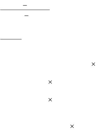
1. Slope coefficient = Error!
=
$5, 400$4,000
10,0006,000
=
$1, 400
4, 000
= $0.35 per machine–hour
Constant = Total cost – (Slope coefficient Quantity of cost driver)
= $5,400 – ($0.35 10,000) = $1,900
= $4,000 – ($0.35 6,000) = $1,900
The cost function based on the two observations is
Maintenance costs = $1,900 + $0.35 Machine–hours
2. The cost function in requirement 1 is an estimate of how costs behave within the relevant
range, not at cost levels outside the relevant range. If there are no months with zero machine–
hours represented in the maintenance account, data in that account cannot be used to estimate the
fixed costs at the zero machine–hours level. Rather, the constant component of the cost function
provides the best available starting point for a straight line that approximates how a cost behaves
within the relevant range.
© 2012 Pearson Education, Inc. Publishing as Prentice Hall. SM Cost Accounting 14/e by Horngren
10–4
10–17 (15 min.) Identifying variable–, fixed–, and mixed–cost functions.
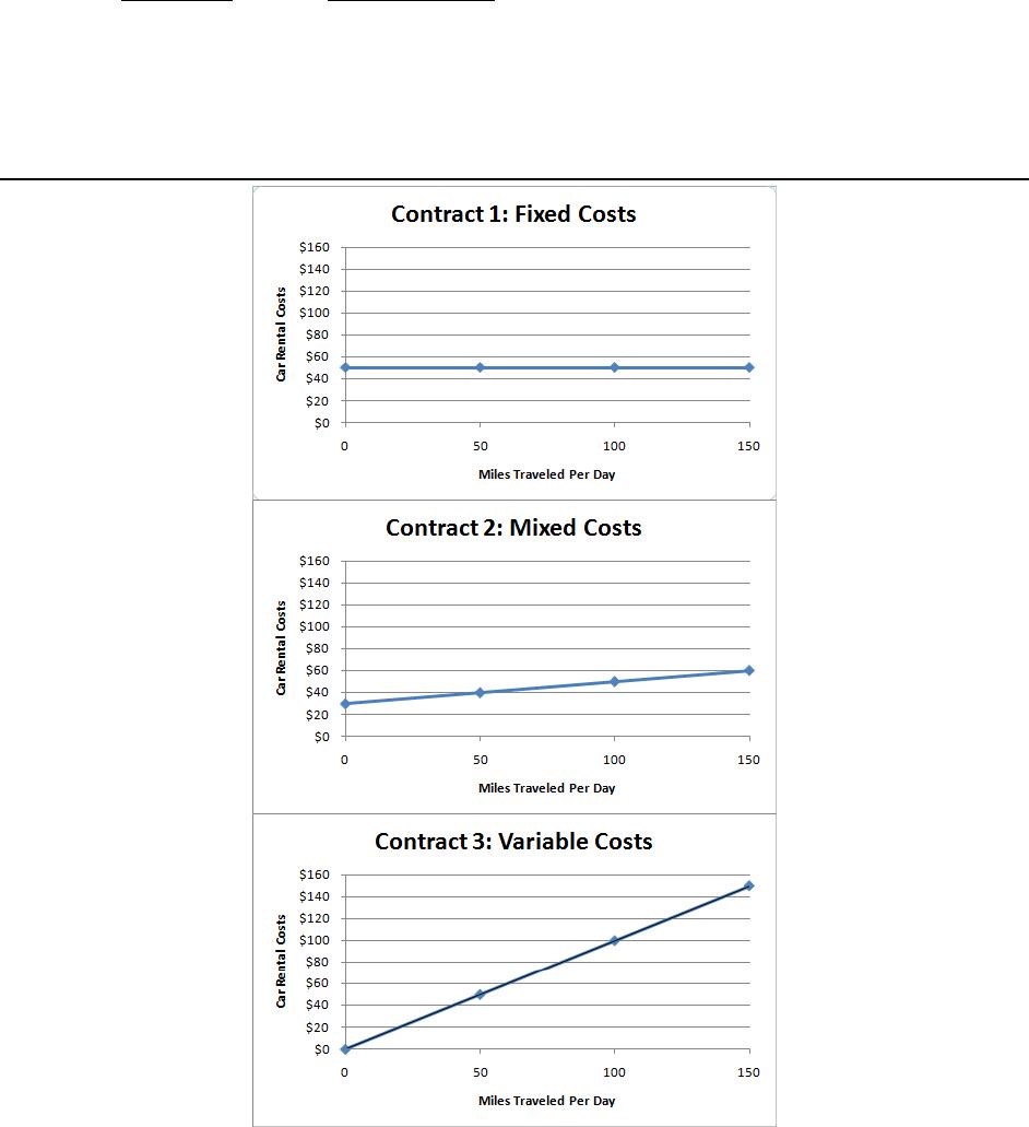
1. See Solution Exhibit 10–17.
2. Contract 1: y = $50
Contract 2: y = $30 + $0.20X
Contract 3: y = $1X
where X is the number of miles traveled in the day.
3.
Contract
Cost Function
1
2
3
Fixed
Mixed
Variable
SOLUTION EXHIBIT 10–17
Plots of Car Rental Contracts Offered by Pacific Corp.
© 2012 Pearson Education, Inc. Publishing as Prentice Hall. SM Cost Accounting 14/e by Horngren
10–5
10–18 (20 min.) Various cost–behavior patterns.
1. K
2. B
3. G
4. J Note that A is incorrect because, although the cost per pound eventually equals a
constant at $9.20, the total dollars of cost increases linearly from that point
onward.
5. I The total costs will be the same regardless of the volume level.
6. L
7. F This is a classic step–cost function.
8. K
9. C
10–19 (30 min.) Matching graphs with descriptions of cost and revenue behavior.
a. (1)
b. (6) A step–cost function.
c. (9)
d. (2)
e. (8)
f. (10) It is data plotted on a scatter diagram, showing a linear variable cost function with
constant variance of residuals. The constant variance of residuals implies that
there is a uniform dispersion of the data points about the regression line.
g. (3)
h. (8)
10–20 (15 min.) Account analysis method.
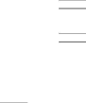
1. Variable costs:
Car wash labor $260,000
Soap, cloth, and supplies 42,000
Water 38,000
Electric power to move conveyor belt 72,000
Total variable costs $412,000
Fixed costs:
Depreciation $ 64,000
Salaries 46,000
Total fixed costs $110,000
Some costs are classified as variable because the total costs in these categories change in
proportion to the number of cars washed in Lorenzo’s operation. Some costs are classified as
fixed because the total costs in these categories do not vary with the number of cars washed. If
the conveyor belt moves regardless of the number of cars on it, the electricity costs to power the
conveyor belt would be a fixed cost.
2. Variable costs per car =
$412,000
80,000
= $5.15 per car
Total costs estimated for 90,000 cars = $110,000 + ($5.15 × 90,000) = $573,500
© 2012 Pearson Education, Inc. Publishing as Prentice Hall. SM Cost Accounting 14/e by Horngren
10–6
10–21 (20 min.) Account analysis
1. The electricity cost is variable because, in each month, the cost divided by the number of
kilowatt hours equals a constant $0.30. The definition of a variable cost is one that remains
constant per unit.
The telephone cost is a mixed cost because the cost neither remains constant in total nor remains
constant per unit.
The water cost is fixed because, although water usage varies from month to month, the cost
remains constant at $60.
2. The month with the highest number of telephone minutes is June, with 1,440 minutes and
$98.80 of cost. The month with the lowest is April, with 980 minutes and $89.60. The
difference in cost ($98.80 – $89.60), divided by the difference in minutes (1,440 – 980) equals
$0.02 per minute of variable telephone cost. Inserted into the cost formula for June:
$98.80 = a fixed cost + ($0.02 × number of minutes used)
$98.80 = a + ($0.02 × 1,440)
$98.80 = a + $28.80
a = $70 monthly fixed telephone cost
Therefore, Java Joe’s cost formula for monthly telephone cost is:
Y = $70 + ($0.02 × number of minutes used)
3. The electricity rate is $0.30 per kw hour
The telephone cost is $70 + ($0.02 per minute)
The fixed water cost is $60
Adding them together we get:
Fixed cost of utilities = $70 (telephone) + $60 (water) = $130
Monthly Utilities Cost = $130 + (0.30 per kw hour) + ($0.02 per telephone min.)
4. Estimated utilities cost = $130 + ($0.30 × 2,200 kw hours) + ($0.02 × 1,500 minutes)
= $130 + $660 + $30 = $820
© 2012 Pearson Education, Inc. Publishing as Prentice Hall. SM Cost Accounting 14/e by Horngren
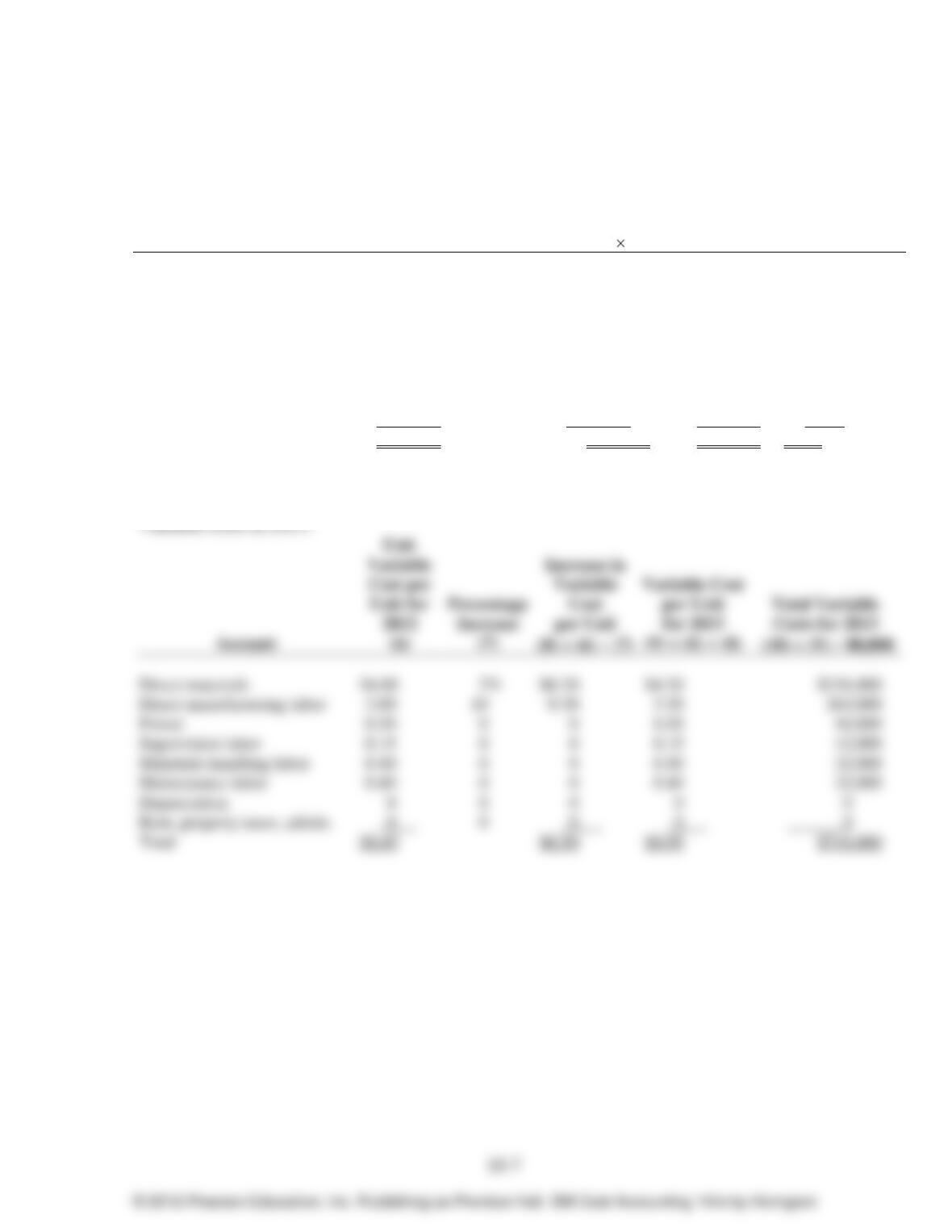
10–22 (30 min.) Account analysis method.
1. Manufacturing cost classification for 2012:
Account
Total
Costs
(1)
% of
Total Costs
That is
Variable
(2)
Variable
Costs
(3) = (1) (2)
Fixed
Costs
(4) = (1) – (3)
Variable
Cost per Unit
(5) = (3) ÷ 75,000
Direct materials
Direct manufacturing labor
Power
Supervision labor
Materials-handling labor
Maintenance labor
Depreciation
Rent, property taxes, admin
$300,000
225,000
37,500
56,250
60,000
75,000
95,000
100,000
100%
100
100
20
50
40
0
0
$300,000
225,000
37,500
11,250
30,000
30,000
0
0
$ 0
0
0
45,000
30,000
45,000
95,000
100,000
$4.00
3.00
0.50
0.15
0.40
0.40
0
0
Total
$948,750
$633,750
$315,000
$8.45
Total manufacturing cost for 2012 = $948,750
5%
0