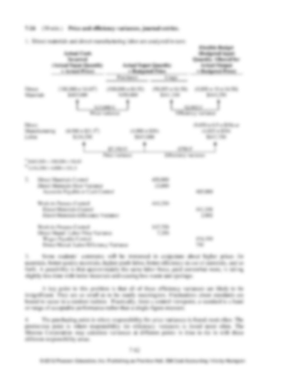
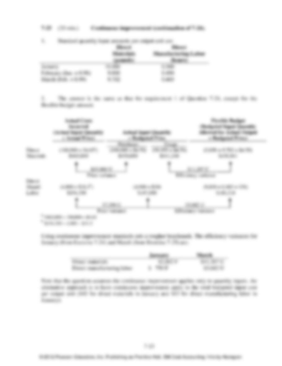
7–1
CHAPTER 7
FLEXIBLE BUDGETS, DIRECT–COST VARIANCES,
AND MANAGEMENT CONTROL
7–1 Management by exception is the practice of concentrating on areas not operating as
expected and giving less attention to areas operating as expected. Variance analysis helps
managers identify areas not operating as expected. The larger the variance, the more likely an
area is not operating as expected.
7–2 Two sources of information about budgeted amounts are (a) past amounts and (b)
detailed engineering studies.
7–3 A favorable variance––denoted F––is a variance that has the effect of increasing
operating income relative to the budgeted amount. An unfavorable variance––denoted U––is a
variance that has the effect of decreasing operating income relative to the budgeted amount.
7–4 The key difference is the output level used to set the budget. A static budget is based on
the level of output planned at the start of the budget period. A flexible budget is developed using
budgeted revenues or cost amounts based on the actual output level in the budget period. The
actual level of output is not known until the end of the budget period.
7–5 A flexible–budget analysis enables a manager to distinguish how much of the difference
between an actual result and a budgeted amount is due to (a) the difference between actual and
budgeted output levels, and (b) the difference between actual and budgeted selling prices,
variable costs, and fixed costs.
7–6 The steps in developing a flexible budget are:
Step 1: Identify the actual quantity of output.
Step 2: Calculate the flexible budget for revenues based on budgeted selling price and
actual quantity of output.
Step 3: Calculate the flexible budget for costs based on budgeted variable cost per output
unit, actual quantity of output, and budgeted fixed costs.
7–7 Four reasons for using standard costs are:
(i) cost management,
(ii) pricing decisions,
(iii) budgetary planning and control, and
(iv) financial statement preparation.
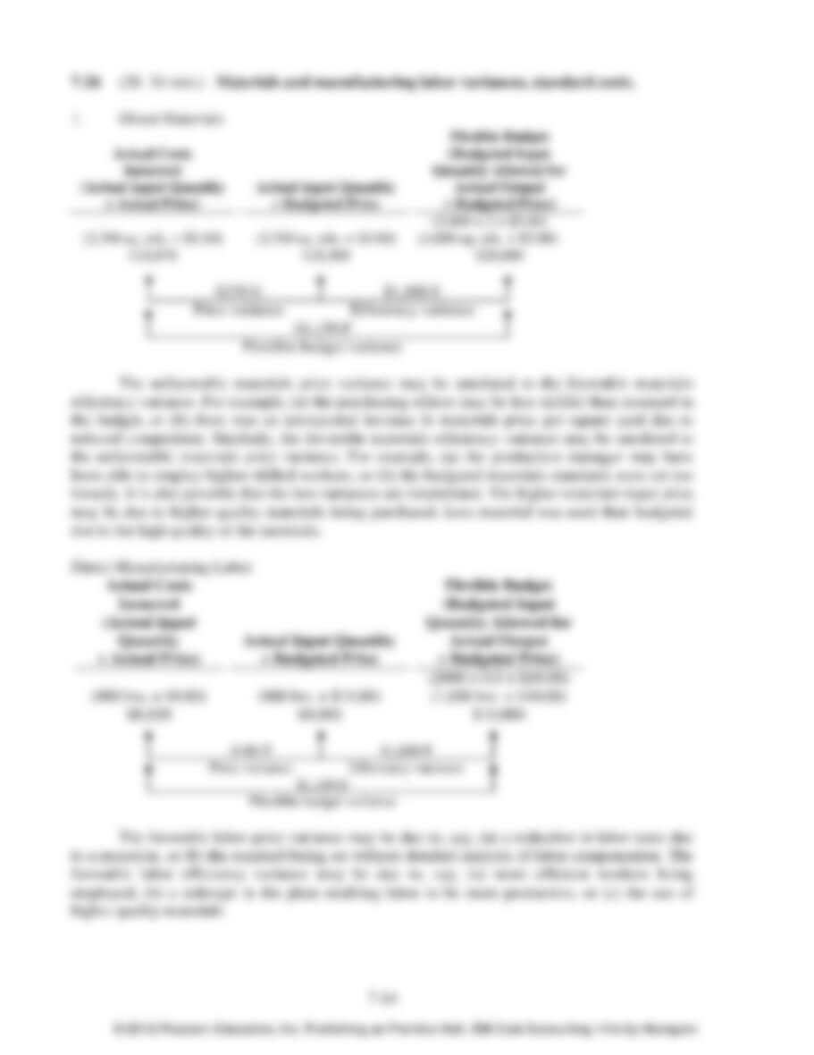
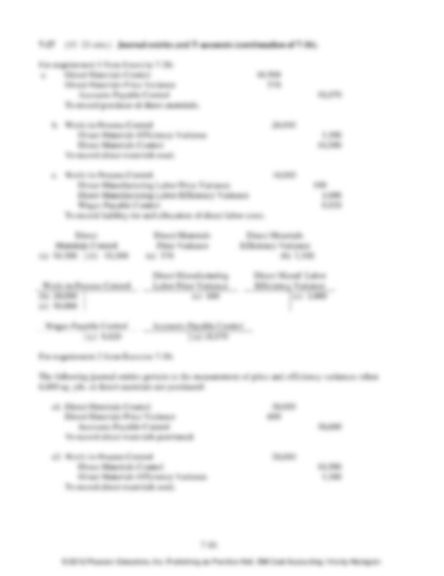
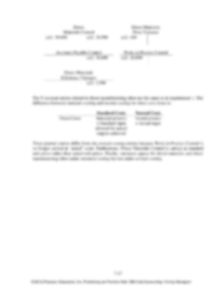
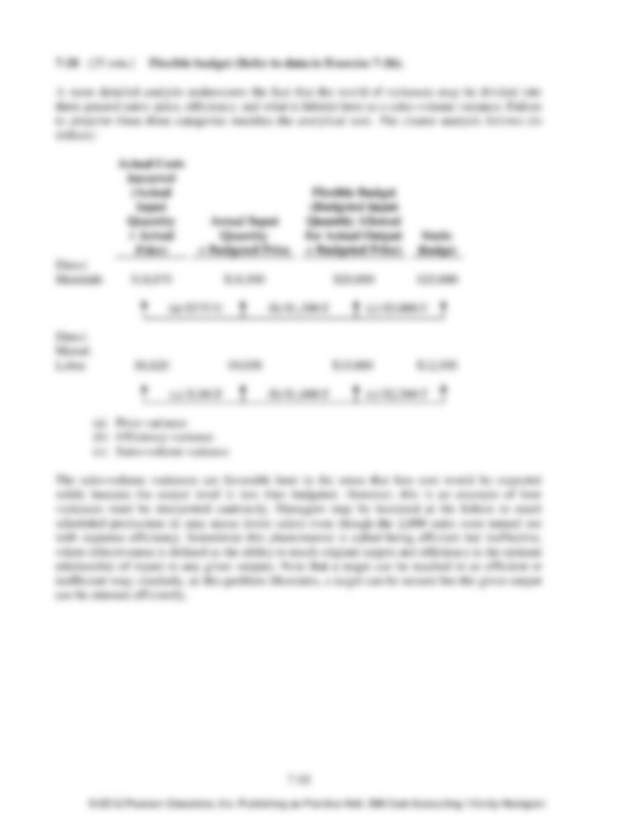
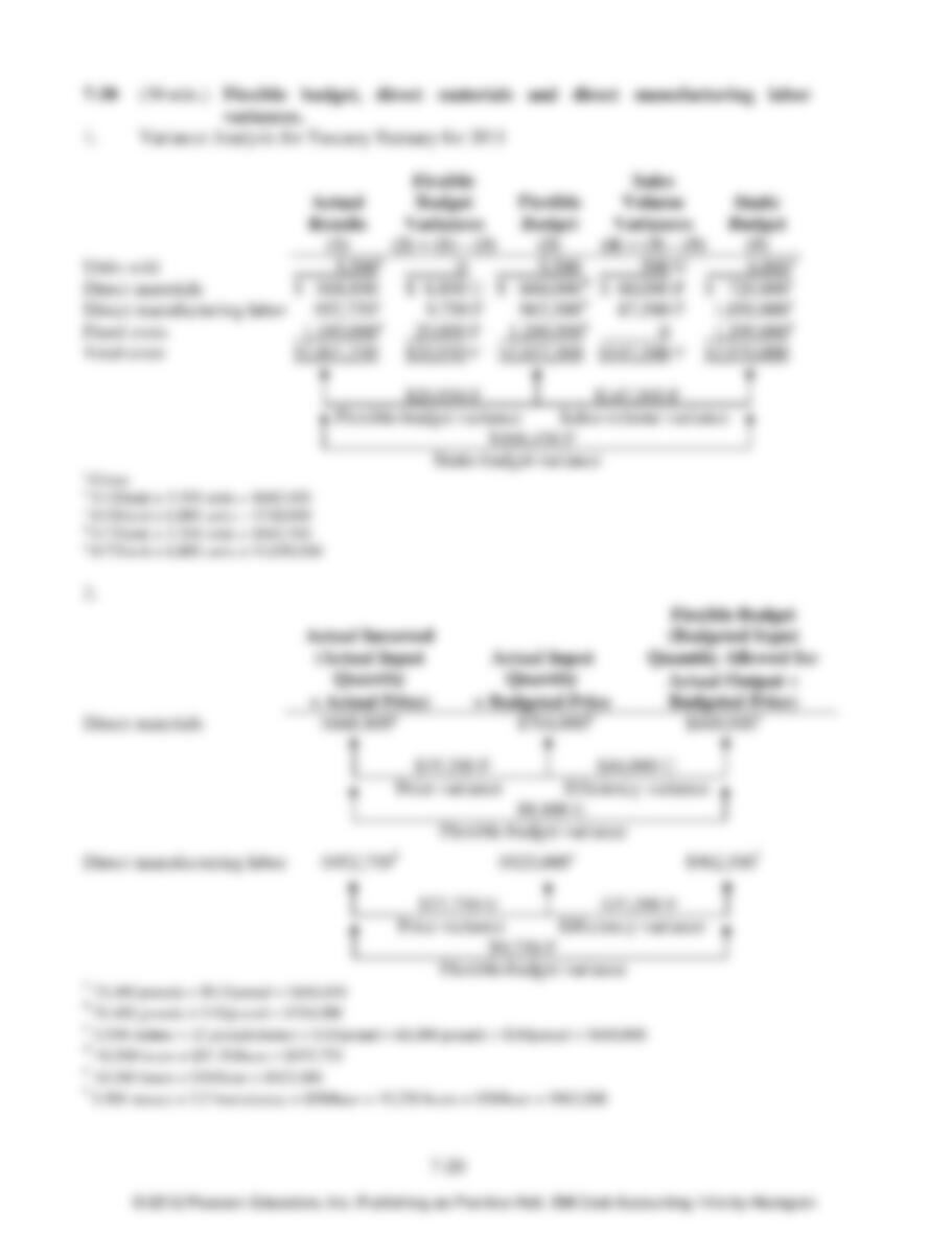
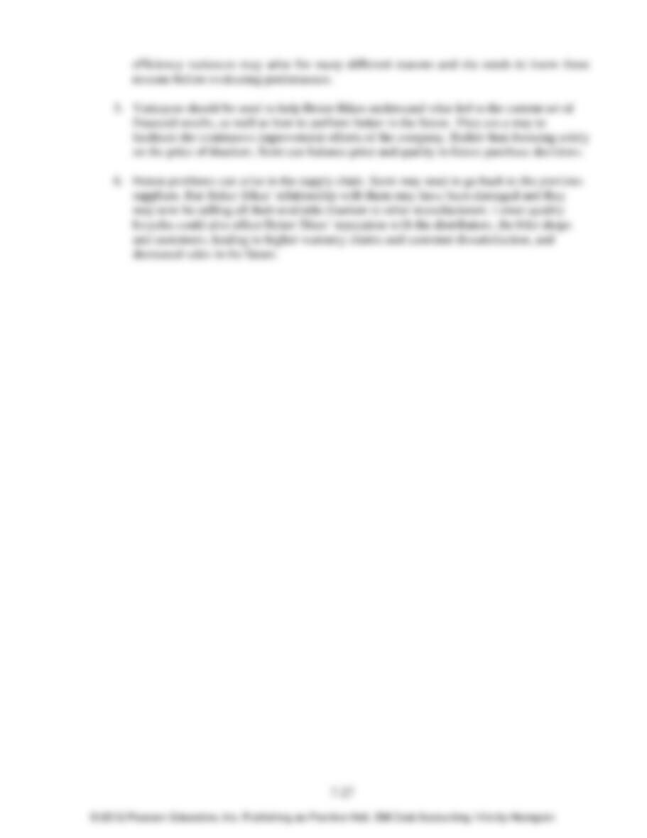
7–8 A manager should subdivide the flexible–budget variance for direct materials into a price
variance (that reflects the difference between actual and budgeted prices of direct materials) and
an efficiency variance (that reflects the difference between the actual and budgeted quantities of
direct materials used to produce actual output). The individual causes of these variances can then
be investigated, recognizing possible interdependencies across these individual causes.
© 2012 Pearson Education, Inc. Publishing as Prentice Hall. SM Cost Accounting 14/e by Horngren

7–2
7–9 Possible causes of a favorable direct materials price variance are:
purchasing officer negotiated more skillfully than was planned in the budget,
purchasing manager bought in larger lot sizes than budgeted, thus obtaining quantity
discounts,
materials prices decreased unexpectedly due to, say, industry oversupply,
budgeted purchase prices were set without careful analysis of the market, and
purchasing manager received unfavorable terms on nonpurchase price factors (such as
lower quality materials).
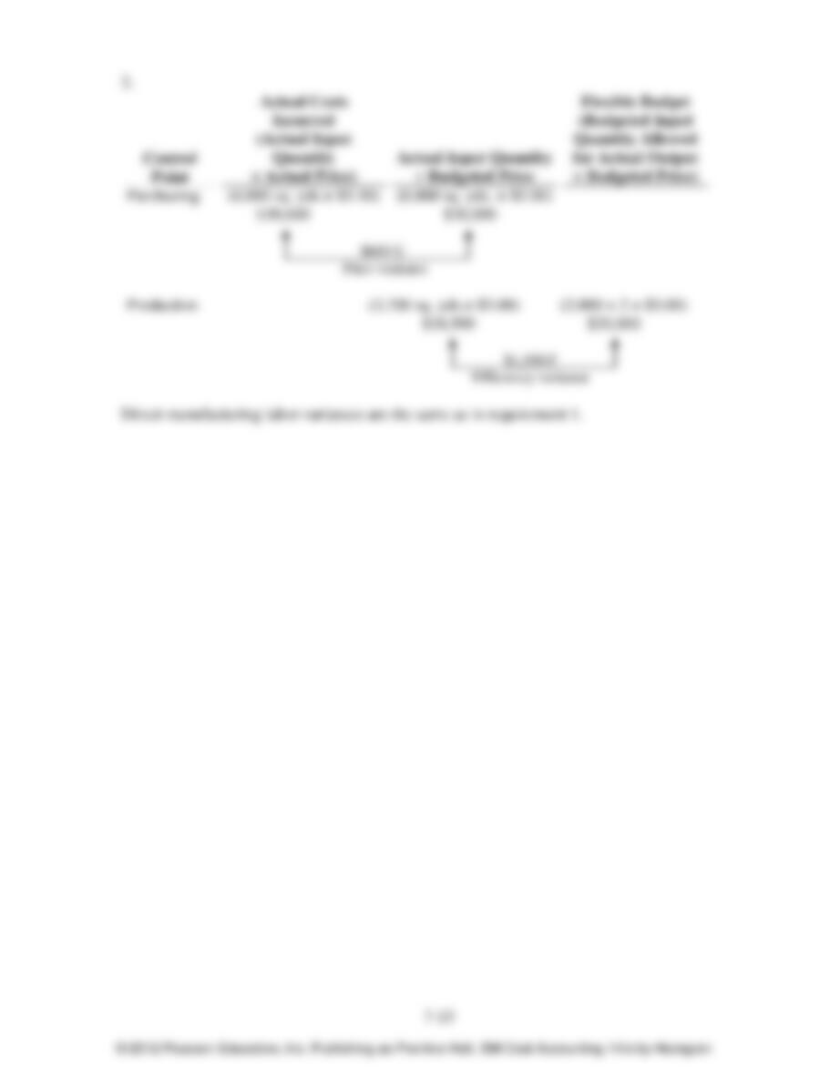
7–10 Some possible reasons for an unfavorable direct manufacturing labor efficiency variance
are the hiring and use of underskilled workers; inefficient scheduling of work so that the
workforce was not optimally occupied; poor maintenance of machines resulting in a high
proportion of non–value–added labor; unrealistic time standards. Each of these factors would
result in actual direct manufacturing labor–hours being higher than indicated by the standard
work rate.
7–11 Variance analysis, by providing information about actual performance relative to
standards, can form the basis of continuous operational improvement. The underlying causes of
unfavorable variances are identified and corrective action taken where possible. Favorable
variances can also provide information if the organization can identify why a favorable variance
occurred. Steps can often be taken to replicate those conditions more often. As the easier changes
are made, and perhaps some standards tightened, the harder issues will be revealed for the
organization to act on—this is continuous improvement.
7–12 An individual business function, such as production, is interdependent with other
business functions. Factors outside of production can explain why variances arise in the
production area. For example:
poor design of products or processes can lead to a sizable number of defects,
marketing personnel making promises for delivery times that require a large number
of rush orders can create production–scheduling difficulties, and
purchase of poor–quality materials by the purchasing manager can result in defects
and waste.
7–13 The plant supervisor likely has good grounds for complaint if the plant accountant puts
excessive emphasis on using variances to pin blame. The key value of variances is to help
understand why actual results differ from budgeted amounts and then to use that knowledge to
promote learning and continuous improvement.
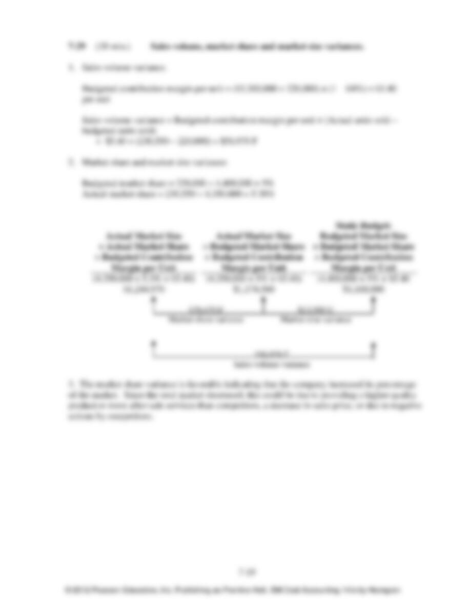
7–14 The sales–volume variance can be decomposed into two parts: a market–share variance
that reflects the difference in budgeted contribution margin due to the actual market share being
different from the budgeted share; and a market–size variance, which captures the impact of
actual size of the market as a while differing from the budgeted market size.
7–15 Evidence on the costs of other companies is one input managers can use in setting the
performance measure for next year. However, caution should be taken before choosing such an
amount as next year‘s performance measure. It is important to understand why cost differences
across companies exist and whether these differences can be eliminated. It is also important to
examine when planned changes (in, say, technology) next year make even the current low–cost
producer not a demanding enough hurdle.
© 2012 Pearson Education, Inc. Publishing as Prentice Hall. SM Cost Accounting 14/e by Horngren
7–3
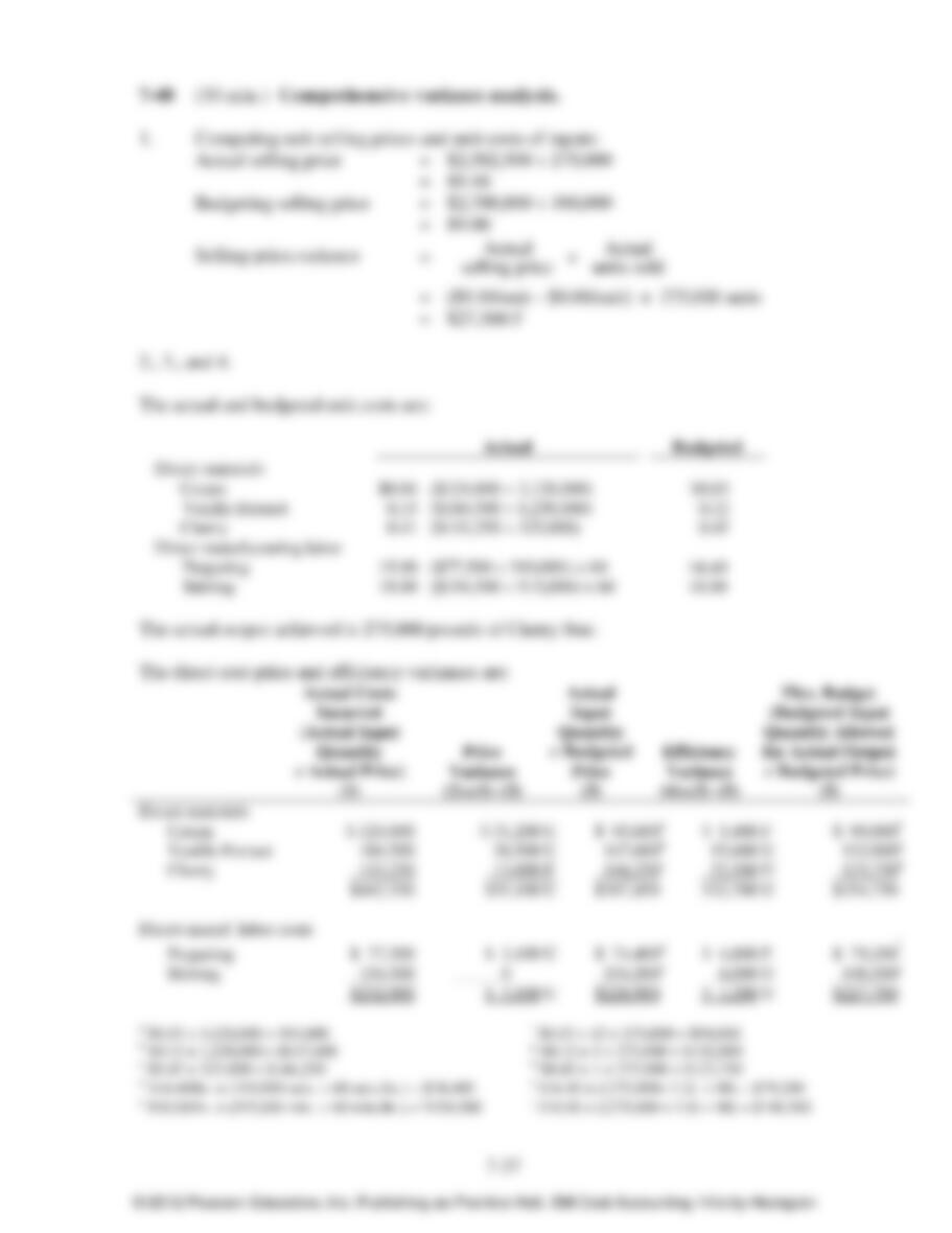
7–16 (20–30 min.) Flexible budget.
Variance Analysis for Brabham Enterprises for August 2012
Actual
Results
(1)
Flexible-
Budget
Variances
(2) = (1) – (3)
Flexible
Budget
(3)
Sales-Volume
Variances
(4) = (3) – (5)
Static
Budget
(5)
Units (tires) sold
2,800g
0
2,800
200 U
3,000g
Revenues
$313,600a
$ 5,600 F
$308,000b
$22,000 U
$330,000c
Variable costs
229,600d
22,400 U
207,200e
14,800 F
222,000f
Contribution margin
84,000
16,800 U
100,800
7,200 U
108,000
Fixed costs
50,000g
4,000 F
54,000g
0
54,000g
Operating income
$ 34,000
$12,800 U
$ 46,800
$ 7,200 U
$ 54,000
$12,800 U $ 7,200 U
Total flexible–budget variance Total sales–volume variance
$20,000 U
Total static–budget variance
a $112 × 2,800 = $313,600
b $110 × 2,800 = $308,000
c $110 × 3,000 = $330,000
d Given. Unit variable cost = $229,600 ÷ 2,800 = $82 per tire
e $74 × 2,800 = $207,200
f $74 × 3,000 = $222,000
g Given
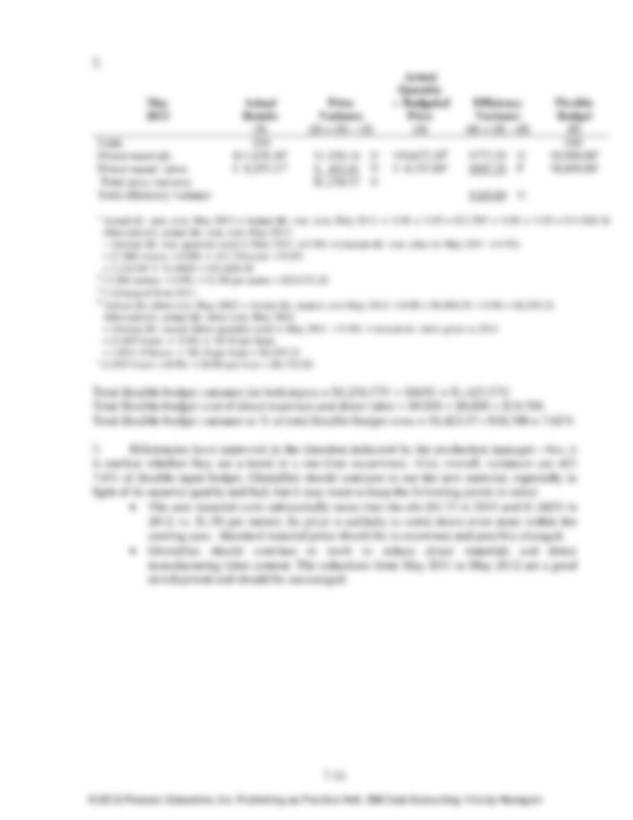
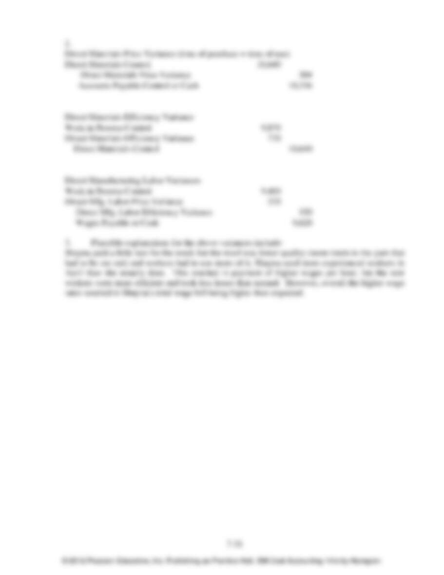
2. The key information items are:
Actual
Budgeted
Units
Unit selling price
Unit variable cost
Fixed costs
2,800
$ 112
$ 82
$50,000
3,000
$ 110
$ 74
$54,000
The total static–budget variance in operating income is $20,000 U. There is both an unfavorable
total flexible–budget variance ($12,800) and an unfavorable sales–volume variance ($7,200).
The unfavorable sales–volume variance arises solely because actual units manufactured
and sold were 200 less than the budgeted 3,000 units. The unfavorable flexible–budget variance
of $12,800 in operating income is due primarily to the $8 increase in unit variable costs. This
increase in unit variable costs is only partially offset by the $2 increase in unit selling price and
the $4,000 decrease in fixed costs.
© 2012 Pearson Education, Inc. Publishing as Prentice Hall. SM Cost Accounting 14/e by Horngren
7–4
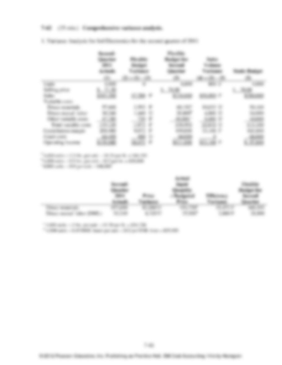
7–17 (15 min.) Flexible budget.
The existing performance report is a Level 1 analysis, based on a static budget. It makes no
adjustment for changes in output levels. The budgeted output level is 10,000 units––direct
materials of $400,000 in the static budget ÷ budgeted direct materials cost per attaché case of
$40.
The following is a Level 2 analysis that presents a flexible–budget variance and a sales–
volume variance of each direct cost category.
Variance Analysis for Connor Company
Actual
Results
(1)
Flexible-
Budget
Variances
(2) = (1) – (3)
Flexible
Budget
(3)
Sales-
Volume
Variances
(4) = (3) – (5)
Static
Budget
(5)
Output units
Direct materials
Direct manufacturing labor
Direct marketing labor
Total direct costs
8,800
$364,000
78,000
110,000
$552,000
0
$12,000 U
7,600 U
4,400 U
$24,000 U
8,800
$352,000
70,400
105,600
$528,000
1,200 U
$48,000 F
9,600 F
14,400 F
$72,000 F
10,000
$400,000
80,000
120,000
$600,000
$24,000 U $72,000 F
Flexible–budget variance Sales–volume variance
$48,000 F
Static–budget variance
The Level 1 analysis shows total direct costs have a $48,000 favorable variance.
However, the Level 2 analysis reveals that this favorable variance is due to the reduction in
output of 1,200 units from the budgeted 10,000 units. Once this reduction in output is taken into
account (via a flexible budget), the flexible–budget variance shows each direct cost category to
have an unfavorable variance indicating less efficient use of each direct cost item than was
budgeted, or the use of more costly direct cost items than was budgeted, or both.
Each direct cost category has an actual unit variable cost that exceeds its budgeted unit
cost:
Actual
Budgeted
Units
Direct materials
Direct manufacturing labor
Direct marketing labor
8,800
$ 41.36
$ 8.86
$ 12.50
10,000
$ 40.00
$ 8.00
$ 12.00
Analysis of price and efficiency variances for each cost category could assist in further the
identifying causes of these more aggregated (Level 2) variances.
© 2012 Pearson Education, Inc. Publishing as Prentice Hall. SM Cost Accounting 14/e by Horngren
7–5
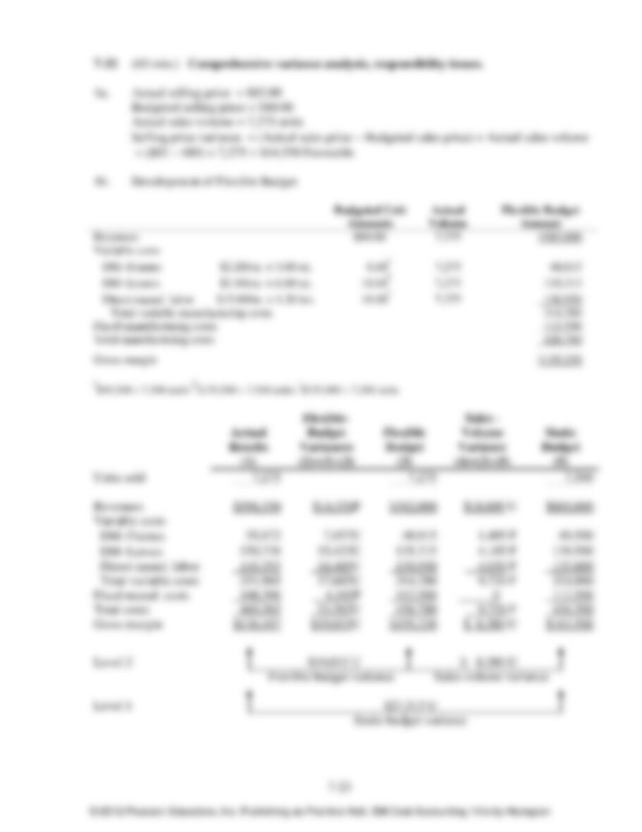
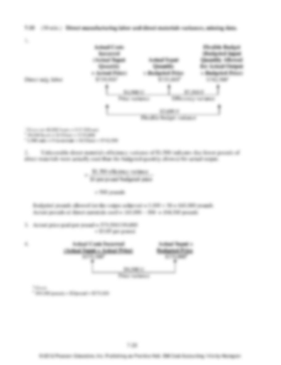
7–18 (25–30 min.) Flexible–budget preparation and analysis.
1. Variance Analysis for Bank Management Printers for September 2012
Level 1 Analysis
Actual
Results
(1)
Static-Budget
Variances
(2) = (1) – (3)
Static
Budget
(3)
Units sold
Revenue
12,000
$252,000a
3,000 U
$48,000 U
15,000
$300,000c
Variable costs
84,000d
36,000 F
120,000f
Contribution margin
Fixed costs
Operating income
168,000
150,000
$ 18,000
12,000 U
5,000 U
$17,000 U
180,000
145,000
$ 35,000
$17,000 U
Total static–budget variance
2. Level 2 Analysis
Actual
Results
(1)
Flexible-
Budget
Variances
(2) = (1) – (3)
Flexible
Budget
(3)
Sales
Volume
Variances
(4) = (3) – (5)
Static
Budget
(5)
Units sold
12,000
0
12,000
3,000 U
15,000
Revenue
$252,000a
$12,000 F
$240,000b
$60,000 U
$300,000c
Variable costs
84,000d
12,000 F
96,000e
24,000 F
120,000f
Contribution margin
168,000
24,000 F
144,000
36,000 U
180,000
Fixed costs
150,000
5,000 U
145,000
0
145,000
Operating income
$ 18,000
$19,000 F
$ (1,000)
$36,000 U
$ 35,000
$19,000 F $36,000 U
Total flexible–budget Total sales–volume
variance variance
$17,000 U
Total static–budget variance
a 12,000 × $21 = $252,000 d 12,000 × $7 = $ 84,000
b 12,000 × $20 = $240,000 e 12,000 × $8 = $ 96,000
c 15,000 × $20 = $300,000 f 15,000 × $8 = $120,000
3. Level 2 analysis breaks down the static–budget variance into a flexible–budget variance
and a sales–volume variance. The primary reason for the static–budget variance being
unfavorable ($17,000 U) is the reduction in unit volume from the budgeted 15,000 to an actual
12,000. One explanation for this reduction is the increase in selling price from a budgeted $20 to
an actual $21. Operating management was able to reduce variable costs by $12,000 relative to
the flexible budget. This reduction could be a sign of efficient management. Alternatively, it
could be due to using lower quality materials (which in turn adversely affected unit volume).
© 2012 Pearson Education, Inc. Publishing as Prentice Hall. SM Cost Accounting 14/e by Horngren
7–6
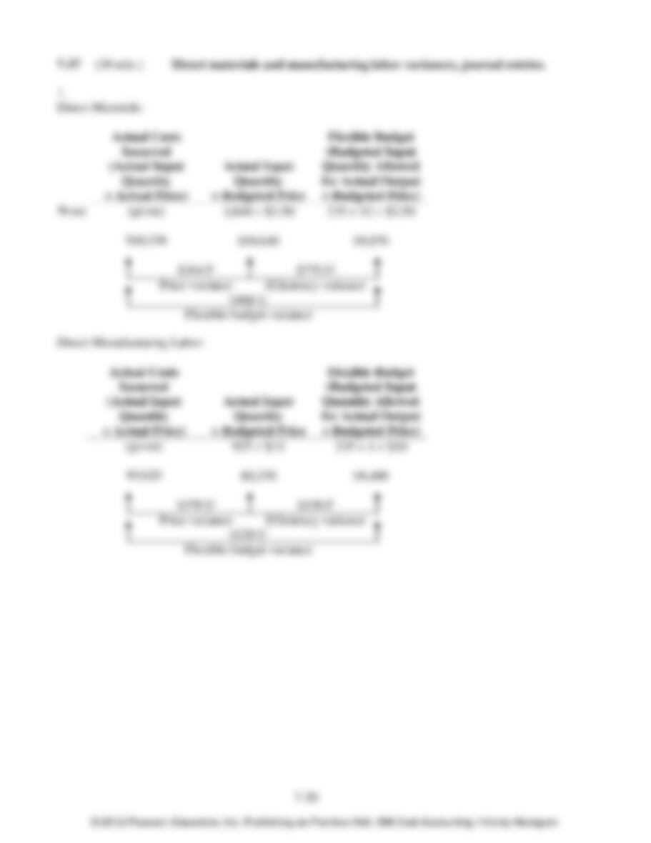
7–19 (30 min.) Flexible budget, working backward.
1. Variance Analysis for The Clarkson Company for the year ended December 31, 2012
Actual
Results
(1)
Flexible-
Budget
Variances
(2)=(1)(3)
Flexible
Budget
(3)
Sales-Volume
Variances
(4)=(3)(5)
Static
Budget
(5)
Units sold
130,000
0
130,000
10,000 F
120,000
Revenues
$715,000
$260,000 F
$455,000a
$35,000 F
$420,000
Variable costs
515,000
255,000 U
260,000b
20,000 U
240,000
Contribution margin
200,000
5,000 F
195,000
15,000 F
180,000
Fixed costs
140,000
20,000 U
120,000
0
120,000
Operating income
$ 60,000
$ 15,000 U
$ 75,000
$15,000 F
$ 60,000
a 130,000 × $3.50 = $455,000; $420,000 120,000 = $3.50
b 130,000 × $2.00 = $260,000; $240,000 120,000 = $2.00
2. Actual selling price: $715,000 130,000 = $5.50
Budgeted selling price: 420,000 ÷ 120,000 = $3.50
Actual variable cost per unit: 515,000 ÷ 130,000 = $3.96
Budgeted variable cost per unit: 240,000 ÷ 120,000 = $2.00
3. A zero total static–budget variance may be due to offsetting total flexible–budget and total
sales–volume variances. In this case, these two variances exactly offset each other:
Total flexible–budget variance $15,000 Unfavorable
Total sales–volume variance $15,000 Favorable
A closer look at the variance components reveals some major deviations from plan.
Actual variable costs increased from $2.00 to $3.96, causing an unfavorable flexible–budget
variable cost variance of $255,000. Such an increase could be a result of, for example, a jump in
direct material prices. Clarkson was able to pass most of the increase in costs onto their
customers—actual selling price increased by 57% [($5.50 – $3.50) $3.50], bringing about an
offsetting favorable flexible-budget revenue variance in the amount of $260,000. An increase in
the actual number of units sold also contributed to more favorable results. The company should
examine why the units sold increased despite an increase in direct material prices. For example,
Clarkson’s customers may have stocked up, anticipating future increases in direct material
prices. Alternatively, Clarkson’s selling price increases may have been lower than competitors’
price increases. Understanding the reasons why actual results differ from budgeted amounts can
help Clarkson better manage its costs and pricing decisions in the future. The important lesson
learned here is that a superficial examination of summary level data (Levels 0 and 1) may be
insufficient. It is imperative to scrutinize data at a more detailed level (Level 2). Had Clarkson
not been able to pass costs on to customers, losses would have been considerable.
$15,000 U
Total flexible-budget variance
$15,000 F
Total sales volume variance
$0
Total static-budget variance
© 2012 Pearson Education, Inc. Publishing as Prentice Hall. SM Cost Accounting 14/e by Horngren
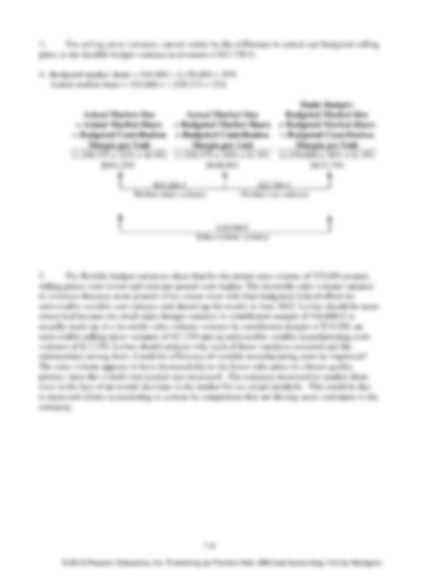
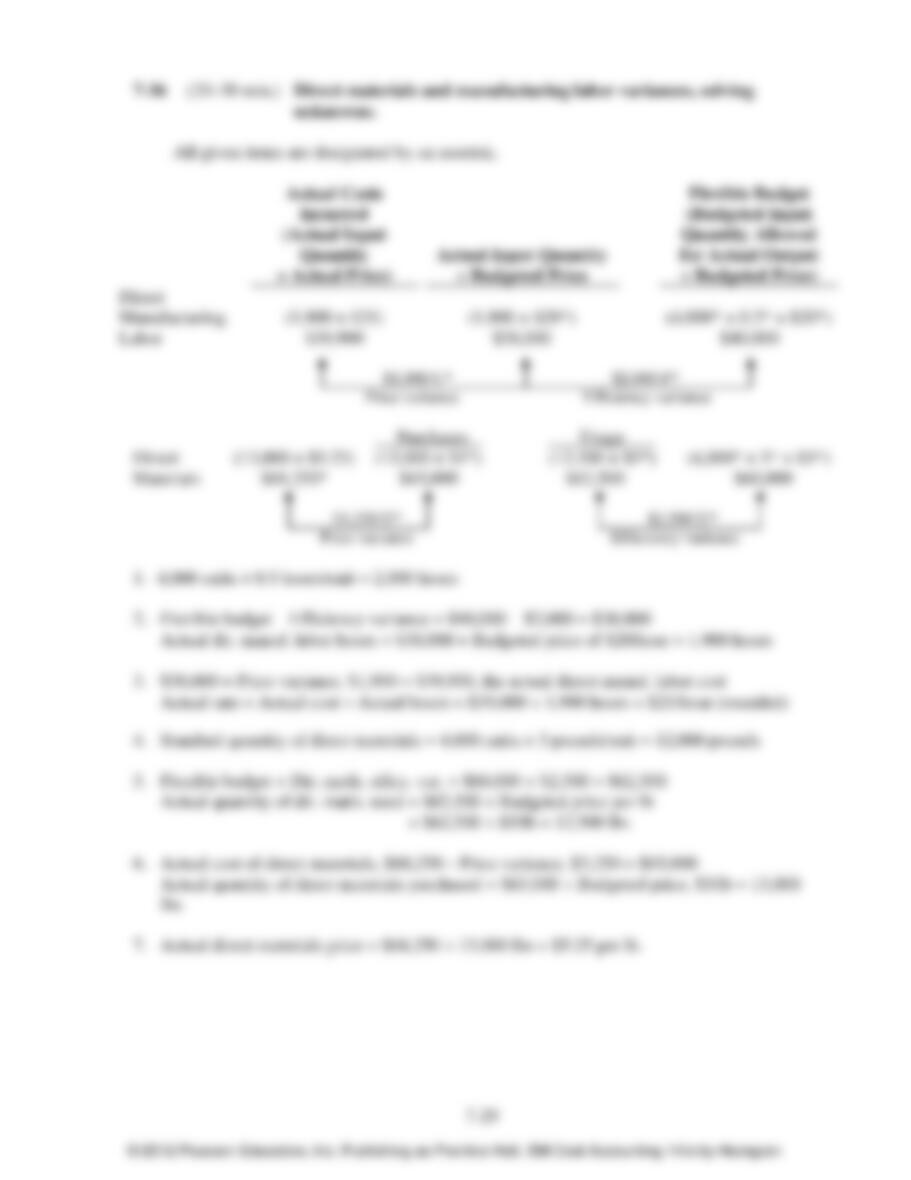
7–20 (30-40 min.) Flexible budget and sales volume variances, market–share and market–size variances.
1. and 2.
Performance Report for Marron, Inc., June 2012
Actual
Flexible Budget
Variances
Flexible Budget
Sales Volume
Variances
Static
Budget
Static
Budget
Variance
Static Budget
Variance as
% of Static
Budget
(1)
(2) = (1) – (3)
(3)
(4) = (3) – (5)
(5)
(6) = (1) – (5)
(7) = (6) (5)
Units (pounds)
355,000
—
355,000
10,000
F
345,000
10,000
F
2.90%
Revenues
$1,917,000
$17,750
U
$1,934,750a
$54,500
F
$1,880,250
$36,750
F
1.95%
Variable mfg. costs
1,260,250
17,750
U
1,242,500b
35,000
U
1,207,500
52,750
U
4.37%