Smhorngren cost accounting 14e CHAPTER 20 INVENTORY MANAGEMENT, JUST-IN-TIME, AND SIMPLIFIED COSTING METHODS

20–1

CHAPTER 20

INVENTORY MANAGEMENT, JUST–IN–TIME,

AND SIMPLIFIED COSTING METHODS

20–1 Cost of goods sold (in retail organizations) or direct materials costs (in organizations with

a manufacturing function) as a percentage of sales frequently exceeds net income as a percentage

of sales by many orders of magnitude. In the Kroger grocery store example cited in the text, cost

of goods sold to sales is 76.8%, and net income to sales is 0.1%. Thus, a 10% reduction in the

ratio of cost of goods sold to sales (76.8 to 69.1% equal to 7.7%) without any other changes can

result in a 7800% increase in net income to sales (0.1% plus 7.7% equal to 7.8%).

20–2 Six cost categories important in managing goods for sale in a retail organization are the

following:

1. purchasing costs;

2. ordering costs;

3. carrying costs;

4. stockout costs;

5. costs of quality; and

6. shrinkage costs

20–3 Five assumptions made when using the simplest version of the EOQ model are:

1. The same quantity is ordered at each reorder point.

2. Demand, ordering costs, carrying costs, and the purchase–order lead time are certain.

3. Purchasing cost per unit is unaffected by the quantity ordered.

4. No stockouts occur.

5. Costs of quality and shrinkage costs are considered only to the extent that these costs affect

ordering costs or carrying costs.

20–4 Costs included in the carrying costs of inventory are incremental costs for such items as

insurance, rent, obsolescence, spoilage, and breakage plus the opportunity cost of capital (or

required return on investment).

20–5 Examples of opportunity costs relevant to the EOQ decision model but typically not

recorded in accounting systems are the following:

1. the return forgone by investing capital in inventory;

2. lost contribution margin on existing sales when a stockout occurs; and

3. lost contribution margin on potential future sales that will not be made to disgruntled

customers.

20–6 The steps in computing the costs of a prediction error when using the EOQ decision

model are:

Step 1: Compute the monetary outcome from the best action that could be taken, given

the actual amount of the cost input.

Step 2: Compute the monetary outcome from the best action based on the incorrect

amount of the predicted cost input.

Step 3: Compute the difference between the monetary outcomes from Steps 1 and 2.

20–2

20–7 Goal congruence issues arise when there is an inconsistency between the EOQ decision

model and the model used for evaluating the performance of the person implementing the model.

For example, if opportunity costs are ignored in performance evaluation, the manager may be

induced to purchase in a quantity larger than the EOQ model indicates is optimal.

20–8 Just–in–time (JIT) purchasing is the purchase of materials (or goods) so that they are

delivered just as needed for production (or sales). Benefits include lower inventory holdings

(reduced warehouse space required and less money tied up in inventory) and less risk of

inventory obsolescence and spoilage.

20–9 Factors causing reductions in the cost to place purchase orders of materials are:

Companies are establishing long–run purchasing agreements that define price and

quality terms over an extended period.

Companies are using electronic links, such as the Internet, to place purchase orders.

Companies are increasing the use of purchase–order cards.

20–10 Disagree. Choosing the supplier who offers the lowest price will not necessarily result in

the lowest total purchase cost to the buyer. This is because the price or purchase cost of the

goods is only one—and perhaps, most obvious—element of cost associated with purchasing and

managing inventories. Other relevant cost items are ordering costs, carrying costs, stockout costs,

quality costs, and shrinkage costs. A low–cost supplier may well impose conditions on the

buyer—such as poor quality, or frequent stockouts, or excessively high inventories—that result

in high total costs of purchase. Buyers must examine all the elements of costs relevant to

inventory management, not just the purchase price.

20–11 Supply–chain analysis describes the flow of goods, services, and information from the

initial sources of materials and services to the delivery of products to consumers, regardless of

whether those activities occur in the same company or in other companies. Sharing of

information across companies enables a reduction in inventory levels at all stages, fewer

stockouts at the retail level, reduced manufacture of product not subsequently demanded by

retailers, and a reduction in expedited manufacturing orders.

20–12 Just–in–time (JIT) production is a ―demand–pull‖ manufacturing system that has the

following features:

Organize production in manufacturing cells,

Hire and retain workers who are multi–skilled,

Aggressively pursue total quality management (TQM) to eliminate defects,

Place emphasis on reducing both setup time and manufacturing cycle time, and

Carefully select suppliers who are capable of delivering quality materials in a timely

manner.

20–13 Traditional normal and standard costing systems use sequential tracking, in which journal

entries are recorded in the same order as actual purchases and progress in production, typically at

four different trigger points in the process.

Backflush costing omits recording some of the journal entries relating to the cycle from

purchase of direct materials to sale of finished goods, i.e., it has fewer trigger points at which

journal entries are made. When journal entries for one or more stages in the cycle are omitted,

20–3

the journal entries for a subsequent stage use normal or standard costs to work backward to

―flush out‖ the costs in the cycle for which journal entries were not made.

20–14 Versions of backflush costing differ in the number and placement of trigger points at

which journal entries are made in the accounting system:

Number of

Journal Entry

Trigger Points

Location in Cycle Where

Journal Entries Made

Version 1

3

Stage A. Purchase of direct materials and incurring of

conversion costs

Stage C. Completion of good finished units of product

Stage D. Sale of finished goods

Version 2

2

Stage A. Purchase of direct materials and incurring of

conversion costs

Stage D. Sale of finished goods

Version 3

2

Stage C. Completion of good finished units of product

Stage D. Sale of finished goods

20–15 Traditional accounting systems cost individual products, and separate product costs from

selling, general, and administrative costs. Lean accounting costs the entire value stream instead

of individual products. Rework costs, unused capacity costs, and common costs that cannot be

reasonably assigned to value streams are excluded from value stream costs. In addition, many

lean accounting systems expense material costs the period they are purchased, rather than storing

them on the balance sheet until the products using the material are sold.

20–16 (20 min.) Economic order quantity for retailer.

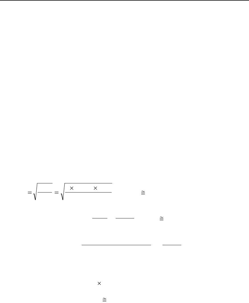
1. D = 10,000 jerseys per year, P = $200, C = $7 per jersey per year

7

200$000,102

C

DP 2

EOQ

= 755.93 756 jerseys

2. Number of orders per year =

EOQ

D

=

756

000,10

= 13.22 14 orders

3.

day workingeach Demand

=

days workingofNumber

D

=

365

000,10

= 27.40 jerseys per day

Purchase lead time = 7 days

Reorder point = 27.40 7

= 191.80 192 jerseys

20–4

20–17 (20 min.) Economic order quantity, effect of parameter changes (continuation of 20–16).

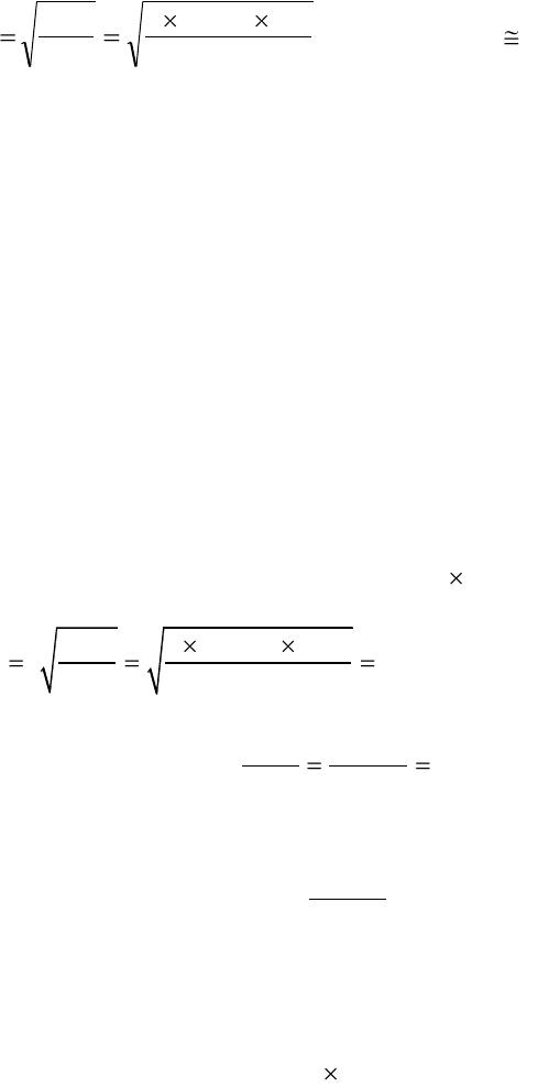
1. D = 10,000 jerseys per year, P = $30, C = $7 per jersey per year

7

30$000,102

C

DP 2

EOQ

= 292.77 jerseys 293 jerseys

The sizable reduction in ordering cost (from $200 to $30 per purchase order) has reduced the

EOQ from 756 to 293.

2. The AT proposal has both upsides and downsides. The upside is potentially higher sales.

FB customers may purchase more online than if they have to physically visit a store. FB would

also have lower administrative costs and lower inventory holding costs with the proposal.

The downside is that AT could capture FB’s customers. Repeat customers to the AT web

site need not be classified as FB customers. FB would have to establish enforceable rules to

make sure it captures ongoing revenues from customers it directs to the AP web site.

There is insufficient information to determine whether FB should accept AT’s proposal.

Much depends on whether FB views AT as a credible, ―honest‖ partner.

20–18 (15 min.) EOQ for a retailer.

1. D = 26,400 yards per year, P = $165, C = 20% $9 = $1.80 per yard per year

226, 400 $165

2 DP

EOQ 2, 200 yards

C$1.80

2. Number of orders per year:

D 26, 400 12 orders per year

EOQ 2, 200

3. Demand each working day = Error!

=

26, 400

250

= 105.60 yards per day

= 528 yards per week (105.60 × 5 days per week)

Purchasing lead time = 2 weeks

Reorder point = 528 yards per week 2 weeks = 1,056 yards

20–5

20–19 (20 min.) EOQ for manufacturer.

1. Relevant carrying costs per part per year:

Required annual return on investment 15% $60 = $ 9

Relevant insurance, materials handling, breakage, etc.

costs per year 6

Relevant carrying costs per part per year $15

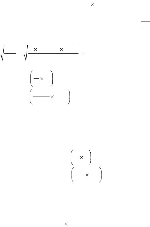
With D = 18,000 parts per year; P = $150; C = $15 per part per year, EOQ for manufacturer is:

2DP 2 18,000 $150

EOQ= 600 units

C $15

2.

Relevant annual

ordering costs

=

D P

Q

=

$150

600

000,18

= $4,500

where Q = 600 units, the EOQ.

3. At the EOQ, total relevant ordering costs and total relevant carrying costs will be exactly

equal. Therefore, total relevant carrying costs at the EOQ = $4,500 (from requirement 2). We

can also confirm this with a direct calculation:

Relevant annual carrying costs

=

C

2

Q

=

$15

2

600

= $4,500

where Q = 600 units, the EOQ.

4. Purchase order lead time is half a month.

Monthly demand is 18,000 units ÷ 12 months = 1,500 units per month.

Demand in half a month is Error! 1,500 units or 750 units.

Lakeland should reorder when the inventory of rotor blades falls to 750 units.

20–6

20–20 (20 min.) Sensitivity of EOQ to changes in relevant ordering and carrying costs.

1. A straightforward approach to the requirement is to construct the following table for

EOQ at relevant carrying and ordering costs. Annual demand is 10,000 units. The formula for the

EOQ model is:

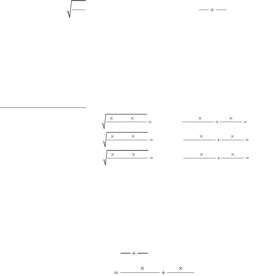
EOQ =

2DPDPQC

and for Relevant Total Costs (RTC) =

C Q 2

where D = demand in units per year

P = relevant ordering costs per purchase order

C = relevant carrying costs of one unit in stock for the time period used for D (one year in

this problem.

Relevant

Carrying

Costs per Unit

per Year

(C)

Relevant

Ordering

Costs per

Purchase

Order

(P)

$10 $400

2 10, 000$40010,000$400895 $10

EOQ = 895, RTC= $8, 944

$10895 2

$20 $200

2 10, 000 $20010,000 $200$47$20

EOQ =447, RTC= $8, 944

$20447 2

$40 $100

2 10, 000 $10010,000 $100224 $40

EOQ =224, RTC= $8, 944

$40224 2

2. For a given demand level, as relevant carrying costs increase and relevant ordering costs

decrease, EOQ becomes smaller. The change in EOQ results in relevant total costs (RTC) being

the same across all three cases. That is, the EOQ offsets the effect on total costs of the increase

in carrying costs and the decrease in ordering costs.

3. If Alpha estimates C = $10 per unit per year and P = $400 per order, then from

requirement 1,

EOQ = 224 units and Relevant Total Cost (RTC) = $8,944

For EOQ = 224 units, C = $20 per unit per year and P = $200 per order,

Relevant total costs (RTC) =

DPQC

Q2

10, 000 $200 224 $20

224 2

= $8,929 + $2,240 = $11,169

The prediction error equals $11,169 – $8,944 = $2,225 which is 25% ($2,225 ÷ $8,944) of the

relevant total cost had there been no prediction error. The error in prediction results is a

significantly higher cost but is still limited, given that the estimate of the carrying cost was half

the actual amount and the estimate of the ordering cost was twice the actual amount. The square

root function dampens the effect of the errors.

20–21 (15 min.) Inventory management and the balanced scorecard.

1. The incremental increase in operating profits from employee cross–training (ignoring the cost

of the training) is:

Increased revenue from higher customer satisfaction ($5,000,000 × 2% × 5) $500,000

Reduced inventory–related costs 100,000

Incremental increase in operating profits (ignoring training costs) $600,000

2. At a cost of $600,000, DSC will be indifferent between current expenditures and increasing

employee cross–training by 5%. Consequently, the most DSC would be willing to pay for this