Signal&system | Course Paper

VIETNAM NATIONAL UNIVERSITY – HOCHIMINH CITY

INTERNATIONAL UNIVERSITY

SCHOOL OF ELECTRICAL ENGINEERING

SIGNALS AND SYSTEMS LABORATORY

Lab 4

Fourier Series

Submitted by

Phan Lê Nhật Tân – EEEEIU18090

Date Submitted: 14/5/2021

Date Performed: 7/5/2021

Lab Section: 4

Course Instructor: Do Ngoc Hung

International University School of Electrical Engineering

SIGNALS AND SYSTEMS LABORATORY EE089

GRADING GUIDELINE FOR LAB REPORT

Number

Content

Score

Comment

1

Format (max 9%)

– Font type

Yes No

– Font size

Yes No

– Lab title

Yes No

– Page number

Yes No

– Table of contents

Yes No

– Header/Footer

Yes No

– List of figures (if exists)

Yes No

– List of tables (if exists)

Yes No

– Lab report structure

Yes No

2

English Grammar and Spelling (max 6%)

– Grammar

Yes No

– Spelling

Yes No

3

Data and Result Analysis (max 85%)

Total Score

Signature:

Date:

International University School of Electrical Engineering

SIGNALS AND SYSTEMS LABORATORY I EE089

Table of Contents

List of Figures …………………………………………………………………………………………………………………… II

List of Tables ……………………………………………………………………………………………………………………. IV

1 Theoretical Background ……………………………………………………………………………………………… 1

1.1 Orthogonality of Complex Exponential Signals ……………………………………………………………. 1

1.2 Complex Exponential Fourier Series …………………………..…………………………………………………. 1

1.3 Trigonometric Fourier Series ………………………………………………………………………………………….. 5

1.4 Fourier Series in the Cosine with Phase Form ……………………………………………………………… 6

1.5 Properties of Fourier Series …………………………………………………………………………………………….. 8

2 Experimental Procedure ……………………………………………………………………………………………… 8

2.1 Experiment 1 ………………………………………………………………………………………………………………………. 8

2.2 Experiment 2 ………………………………………………………………………………………………………………………. 9

2.3 Experiment 3 ……………………………………………………………………………………………………………………. 10

2.4 Experiment 4 ……………………………………………………………………………………………………………………. 12

2.5 Experiment 5 ……………………………………………………………………………………………………………………. 14

2.6 Experiment 6 ……………………………………………………………………………………………………………………. 15

3 Experimental Results …………………………………………………………………………………………………. 32

3.1 Experiment 1 ……………………………………………………………………………………………………………………. 32

3.2 Experiment 2 ……………………………………………………………………………………………………………………. 32

3.3 Experiment 3 ……………………………………………………………………………………………………………………. 33

3.4 Experiment 4 ……………………………………………………………………………………………………………………. 37

3.5 Experiment 5 ……………………………………………………………………………………………………………………. 37

3.6 Experiment 6 ……………………………………………………………………………………………………………………. 38

4 Discussion of Results ………………………………………………………………………………………………….. 62

International University School of Electrical Engineering

SIGNALS AND SYSTEMS LABORATORY II EE089

List of Figures

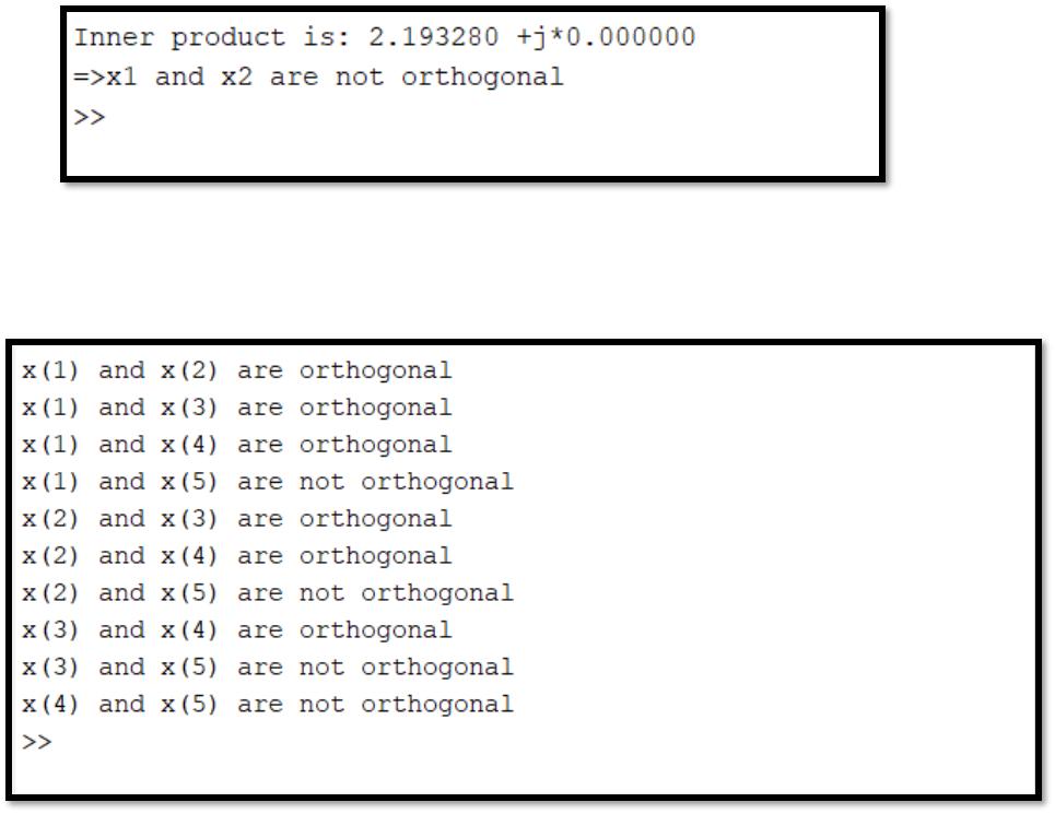
Figure 1. Result of Problem 1 ………………………………………………………………………………………………… 32

Figure 2. Result of Problem 2 ………………………………………………………………………………………………… 32

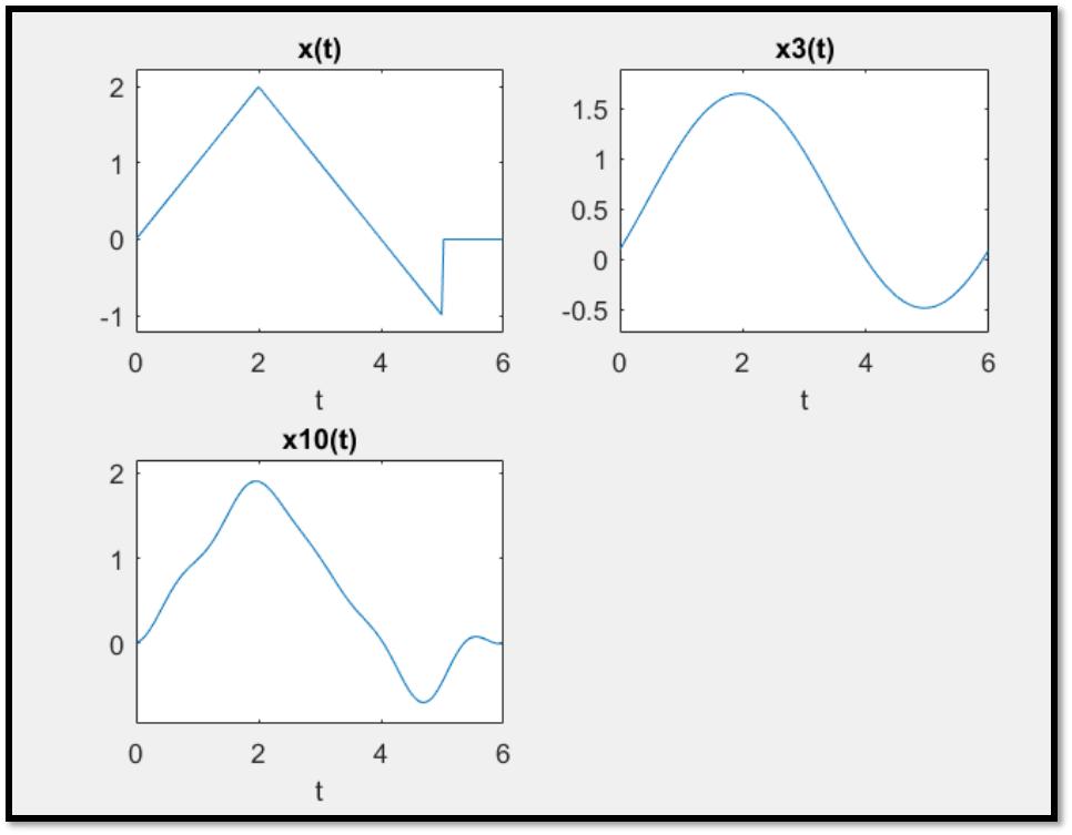
Figure 3. Plotting Approximated Signals Problem 3a ……………………………………………………….. 33

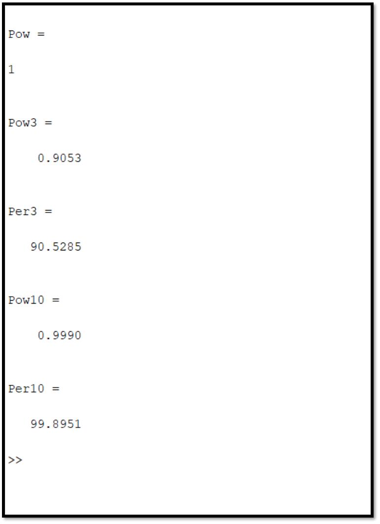
Figure 4. The result percentage of Problem 3.a ………………………………………………………………….. 34

Figure 5. Plotting Approximated Signals Problem 3b ……………………………………………………….. 35

Figure 6. The result percentage of Problem 3b ………………………………………………………………….. 36

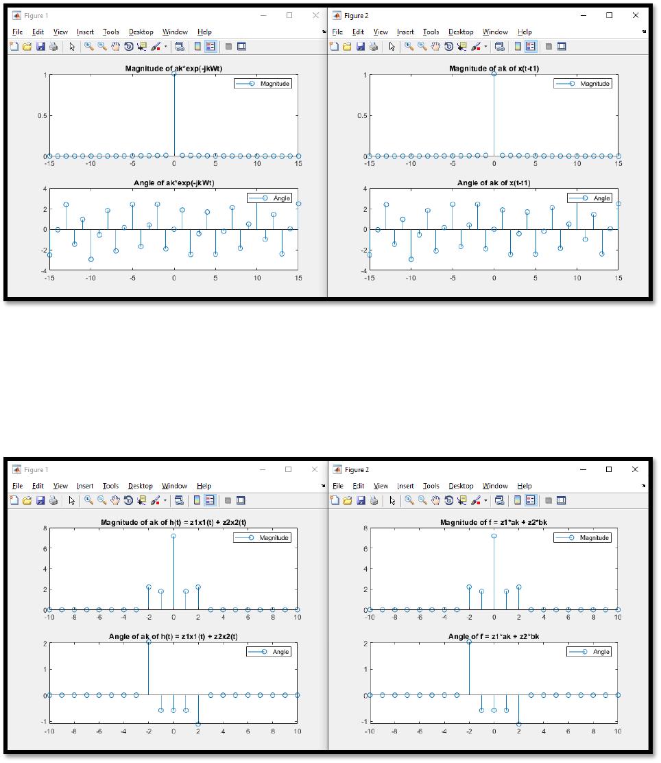
Figure 7. Result of Problem 4 ………………………………………………………………………………………………… 37

Figure 8. Result of Problem 5 ………………………………………………………………………………………………… 37

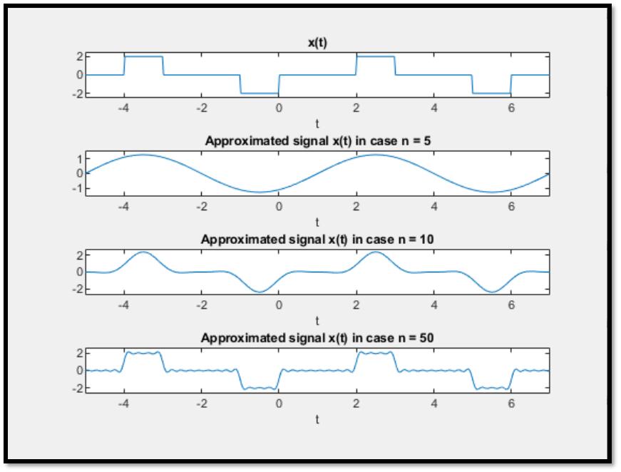
Figure 9. Plotting Approximated Signals Problem 6a ……………………………………………………….. 38

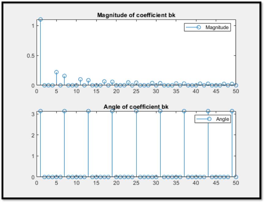
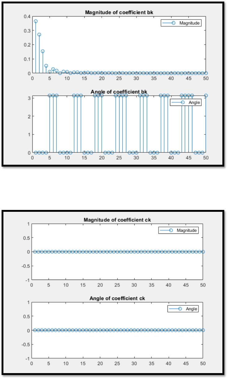
Figure 10. Plotting Magnitude and Phase of Coefficient bk Problem 6a …………………………. 39

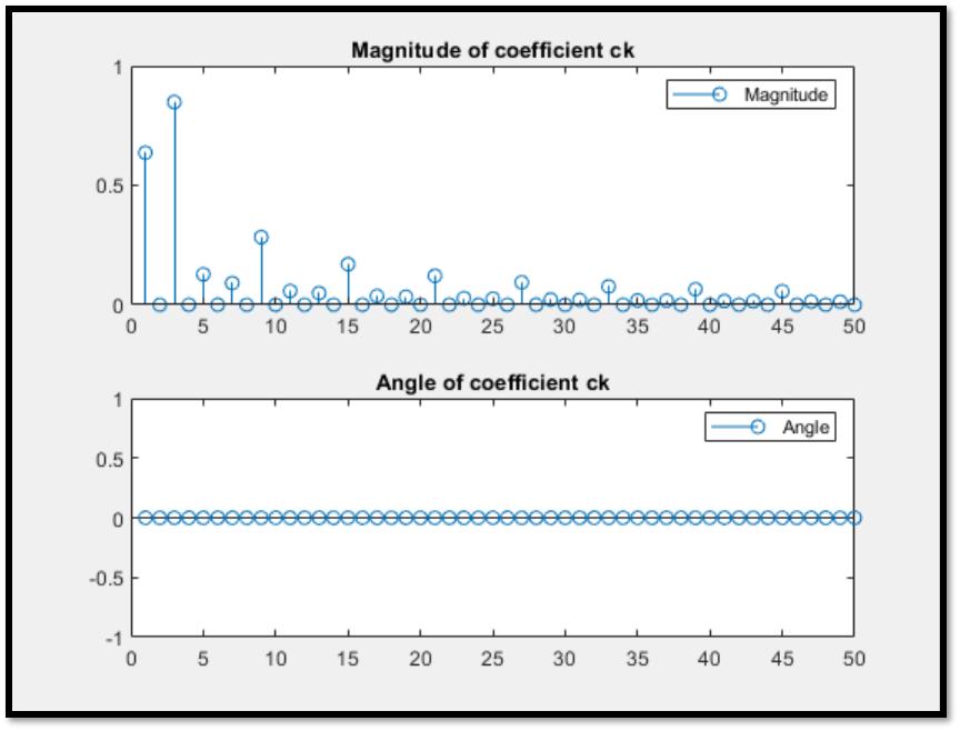
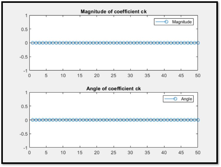
Figure 11. Plotting Magnitude and Phase of Coefficient ck Problem 6a …………………………. 40

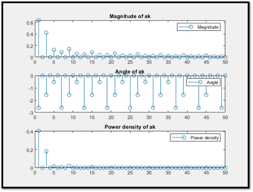
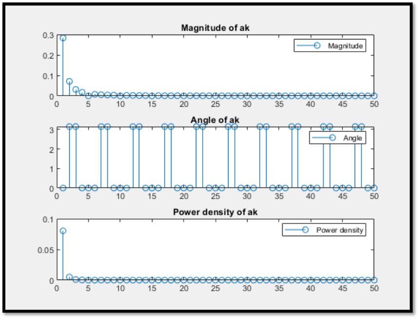
Figure 12. Plotting line spectra ……………………………………………………………………………………………… 41

Figure 13 ……………………………………………………………………………………………………………………………………. 42

Figure 14 ……………………………………………………………………………………………………………………………………. 43

Figure 15. Plotting Magnitude and Phase of Coefficient bk Problem 6b ………………………… 44

Figure 16. Plotting Magnitude and Phase of Coefficient ck Problem 6b …………………………. 44

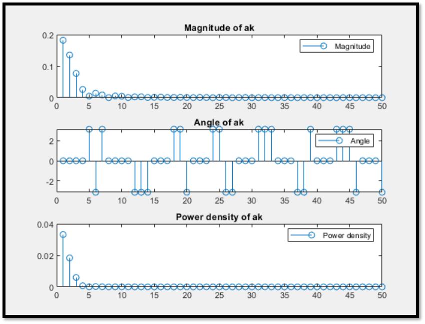
Figure 17. Plotting Line Spectra…………………………………………………………………………………………….. 45

Figure 18 ……………………………………………………………………………………………………………………………………. 46

Figure 19 ……………………………………………………………………………………………………………………………………. 47

Figure 20. Plotting Magnitude and Phase of Coefficient bk Problem 6c …………………………. 48

Figure 21. Plotting Magnitude and Phase of Coefficient ck Problem 6c …………………………. 49

Figure 22. Plotting Line Spectra…………………………………………………………………………………………….. 50

Figure 23 ……………………………………………………………………………………………………………………………………. 51

Figure 24 ……………………………………………………………………………………………………………………………………. 52

Figure 25. Plotting Magnitude and Phase of Coefficient bk Problem 6d ………………………… 53

Figure 26. Plotting Magnitude and Phase of Coefficient ck Problem 6d …………………………. 54

Figure 27. Plotting Line Spectra…………………………………………………………………………………………….. 55

Figure 28 ……………………………………………………………………………………………………………………………………. 56

Figure 29 ……………………………………………………………………………………………………………………………………. 57

International University School of Electrical Engineering

SIGNALS AND SYSTEMS LABORATORY III EE089

Figure 30. Plotting Magnitude and Phase of Coefficient bk Problem 6e …………………………. 58

Figure 31.Plotting Magnitude and Phase of Coefficient ck Problem 6e …………………………. 59

Figure 32.Plotting Line Spectra ……………………………………………………………………………………………… 60

Figure 33 ……………………………………………………………………………………………………………………………………. 61

International University School of Electrical Engineering

SIGNALS AND SYSTEMS LABORATORY IV EE089

List of Tables

No table of figures entries found.

International University School of Electrical Engineering

SIGNALS AND SYSTEMS LABORATORY 1 EE089

1 Theoretical Background

1.1 Orthogonality of Complex Exponential Signals

Suppose that xm(t) and xk(t) are two complex-valued continuous-time periodic signals

with period T. These two signals are orthogonal if their inner product is zero. The inner

product of xm(t) and xk(t) is given by

I=∫xm(𝑡)

t0+T

t0 𝑥∗k(𝑡)𝑑𝑡 (1)

where x*k(t) is the complex conjugate of xk(t).

If I = 0 for m  k, the signal x t m ( ) and ( ) k x t are orthogonal.

Suppose now that xm(t) = ejmΩ0t, xk(t) = ejkΩ0t, k, m  Z. These two signals are orthogonal

as:

I=∫ (𝑒𝑗𝑚Ω0𝑡𝑒−𝑗𝑘Ω0𝑡)

T

0𝑑𝑡 =∫ (𝑒𝑗(𝑚−𝑘)Ω0𝑡)

T

0𝑑𝑡= {0,𝑘≠𝑚

𝑇,𝑘=𝑚 (2)

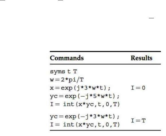
In order to verify the orthogonality of complex exponential signals, consider the signals

𝑥(𝑡)= 𝑒−𝑗3(2𝜋

𝑇)𝑡 and 𝑦(𝑡)= 𝑒𝑗5(2𝜋

𝑇)𝑡.

In this case, the complex conjugate of y(t) is 𝑦∗(𝑡)= 𝑒−𝑗5(2𝜋

𝑇)𝑡

The following table describes the solution of the above example.

1.2 Complex Exponential Fourier Series

Suppose that a signal x(t) is defined in the time interval t0, t0 + T. Then, x(t) is

expressed in exponential Fourier series form as

International University School of Electrical Engineering

SIGNALS AND SYSTEMS LABORATORY 2 EE089

x(t)=∑ 𝑎𝑘𝑒𝑗𝑘Ω0𝑡,𝑡 ∈[𝑡0,𝑡0+𝑇]

∞

k=−∞ , (3)

where 0 is the fundamental frequency, and is given by 0 = 2/T , and t0, T, are real

numbers.

The terms ak are given by 𝑎𝑘=1

𝑇∫𝑥(𝑡)𝑒−𝑗𝑘Ω0𝑡

t0+T

t0 𝑑𝑡, (4)

where the orthogonality property of complex exponential signals was taken into account to

derive ak. The complex coefficients ak are called complex exponential Fourier series

coefficients, while a0 is real number and is called the constant or DC component.

Each coefficient ak corresponds to the projection of the signal x(t) on the kth orthogonal

component 𝑒𝑗𝑘Ω0𝑡, and indicates the spectrum content of the signal x(t) at the frequency k0,

which is known as the kth harmonic. The Fourier series expansion is valid only in the interval

t0, t0 + T, and the value of T defines the fundamental frequency 0. As the Fourier series

coefficients represent the signal in the frequency domain, we refer to them as the spectral

coefficients of the signal.

Example 1:

Expand in complex exponential Fourier series the signal

x(t)=𝑒−𝑡,0 ≤𝑡 ≤3

Solution:

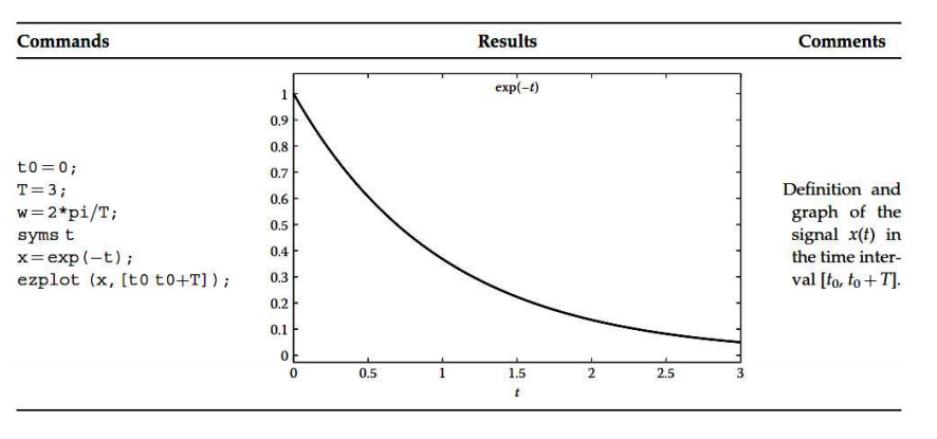
The first thing that needs to be done is to define the quantities t0 = 0, T = 3, and 0 =

2/T. Moreover, the signal x(t) is defined as symbolic expression.

International University School of Electrical Engineering

SIGNALS AND SYSTEMS LABORATORY 3 EE089

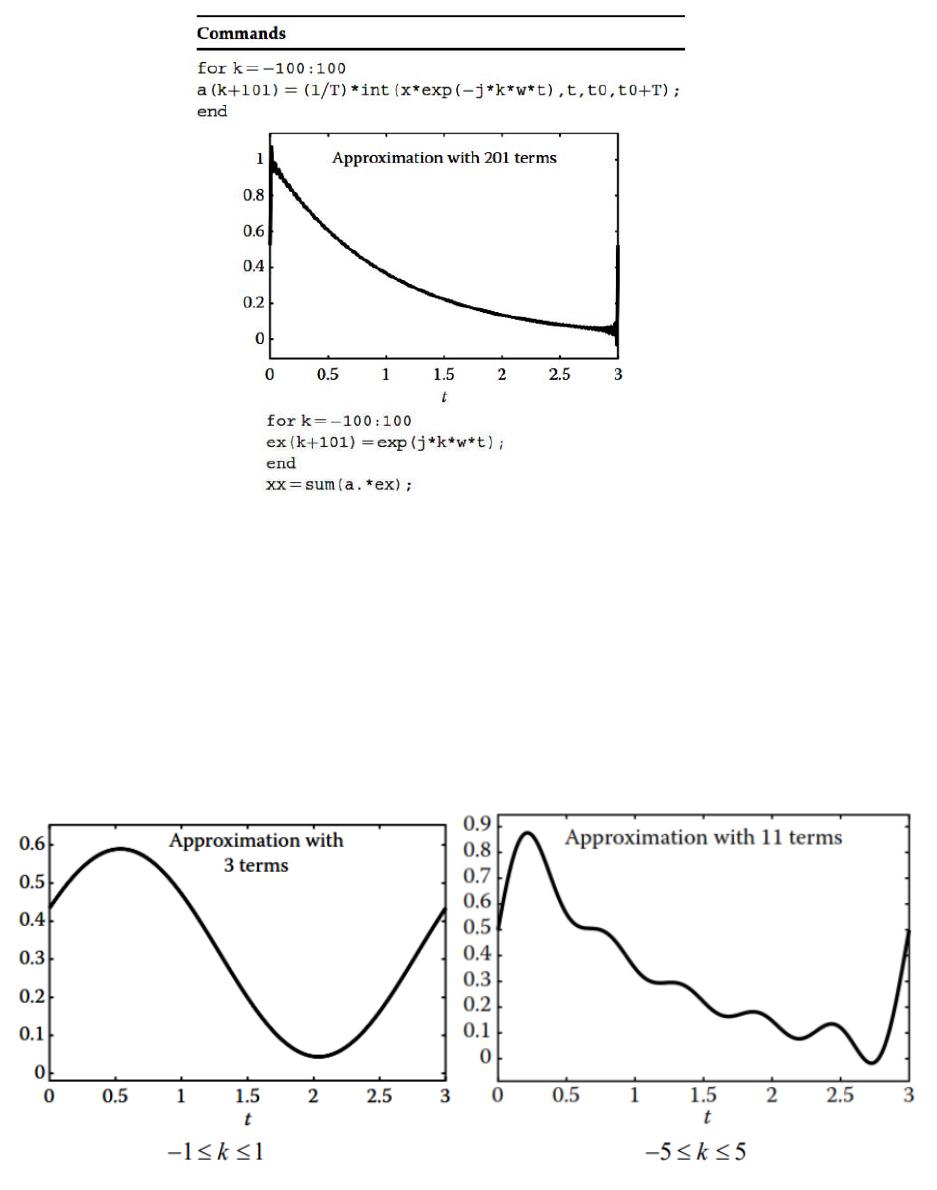
Afterward, the coefficients ak are computed according to Equation (4). Looking into

Equation (3), we observe that infinite Fourier coefficients a have to be calculated. Of course,

this computation cannot be done in an analytical way. Fortunately, as the index k approaches

toward + or toward −, the Fourier coefficients ak are approaching zero. Thus, x(t) can be

satisfactorily approximated by using a finite number of complex exponential Fourier series

terms. Consequently, by computing the coefficients ak for −100  k  100, i.e., by using the

first 201 complex exponential terms, a good approximation of xx(t) is expected. The

approximate signal is denoted by xx t( ) , and is computed by

xx(t)= ∑ 𝑎𝑘𝑒𝑗𝑘Ω0𝑡,𝑡 ∈[𝑡0,𝑡0+𝑇]

K

k=−K

International University School of Electrical Engineering

SIGNALS AND SYSTEMS LABORATORY 4 EE089

The plotted signal xx(t) that is computed with the use of the complex exponential

Fourier series is almost identical with the original signal x(t). In order to understand the

importance of the number of terms used for the approximation of the original signal x(t), the

approximate signal xx(t) is constructed for different values of k. First, the signal x(t) is

approximated by three exponential terms, i.e., the coefficients ak are computed for −1  k 

1 and −5  k  5

From the above analysis, it is clear that when many exponential terms are being

considered in the construction of the approximate signal, a better approximation of the

International University School of Electrical Engineering

SIGNALS AND SYSTEMS LABORATORY 5 EE089

original signal is obtained. As illustrated in the beginning of the example, when 201 terms

were used for the construction of the approximate signal, the obtained approximation was

very good.

1.3 Trigonometric Fourier Series

In this section, we introduce a second form of Fourier series. Suppose that a signal x(t)

is defined in the time interval t0, t0 + T. Then x(t), by using the trigonometric Fourier series,

can be expressed in the time interval t0, t0 + T as a sum of sinusoidal signals, namely sines

and cosines, where each signal has frequency k0 The mathematical expression is

x(t)=𝑎0+∑ 𝑏𝑘cos(𝑘



0𝑡)+∑𝑐𝑘sin(𝑘



0𝑡).

∞

k=1

∞

k=1 (5)

The coefficients of the trigonometric Fourier series are computed by

𝑎0=1

𝑇∫𝑥(𝑡)

t0+T

t0 𝑑𝑡, (6)

𝑏𝑛=2

𝑇∫𝑥(𝑡)cos(𝑛



0𝑡)

t0+T

t0 𝑑𝑡,𝑛=1,2,… (7)

𝑐𝑛=2

𝑇∫𝑥(𝑡)sin(𝑛



0𝑡)

t0+T

t0 𝑑𝑡,𝑛=1,2,… (8)

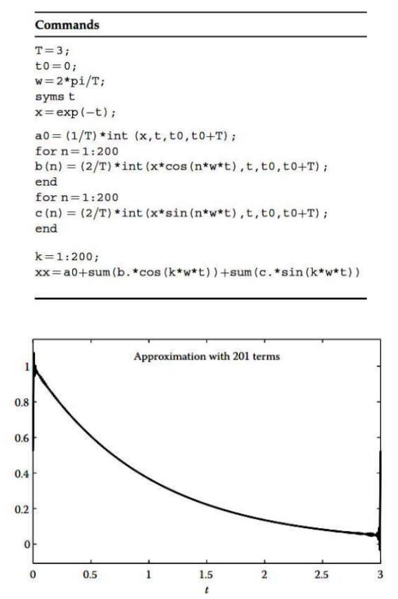
Example 2:

The signal that will be expanded is the same signal used at the previous example.

Solution:

International University School of Electrical Engineering

SIGNALS AND SYSTEMS LABORATORY 6 EE089

1.4 Fourier Series in the Cosine with Phase Form

A third form of Fourier series is derived by using the trigonometric property

𝑏𝑛cos(𝑛



0𝑡)+ 𝑐𝑛sin(𝑛



0𝑡) = 𝐴𝑘cos(𝑘



0𝑡+ 𝜃𝑘) (9)

Here, the signal x(t) (which is defined in the time interval t0, t0 + T is expressed as

x(t)=𝑎0+∑𝐴𝑘cos(𝑘



0𝑡+ 𝜃𝑘)

∞

k=1 (10)

Thus, the signal x(t) is expanded in a sum of sinusoids with different amplitudes and

phases. The coefficients are given by

International University School of Electrical Engineering

SIGNALS AND SYSTEMS LABORATORY 7 EE089

𝑎0=1

𝑇∫𝑥(𝑡)

t0+T

t0 𝑑𝑡, (11)

𝐴𝑘= √𝑏𝑘

2+ 𝑐𝑘

2,𝑘=1,2,… (12)

𝜃𝑘= {tan−1(−𝑐𝑘

𝑏𝑘)= −tan−1(𝑐𝑘

𝑏𝑘),𝑘=1,2,…,𝑤ℎ𝑒𝑛 𝑏𝑘≥0

𝜋+ tan−1(−𝑐𝑘

𝑏𝑘),𝑘=1,2,…,𝑤ℎ𝑒𝑛 𝑏𝑘0 (13)

Due to the two-part definition of the phases k, it is more suitable and secure to use the

atan2 command instead of atan, when computing the phase angle.

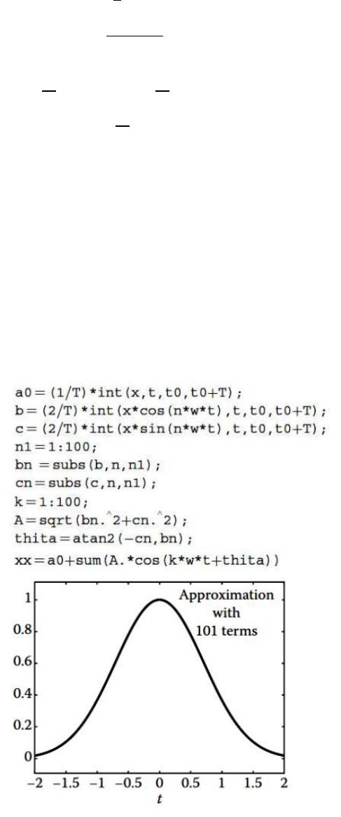
Example 3:

Expand the signal 𝑥(𝑡)= 𝑒−𝑡2, −2  t  2 in the Fourier series in the cosine with phase

form.

Solution:

International University School of Electrical Engineering

SIGNALS AND SYSTEMS LABORATORY 8 EE089

1.5 Properties of Fourier Series

Periodic signal

• Infinite energy

• Finite average power

Parseval’s relation for power signals

𝑃𝑥= 1

𝑇∫|𝑥(𝑡)|2𝑑𝑡

𝑇=∑ |𝑎𝑘|2

∞

k=−∞ (14)

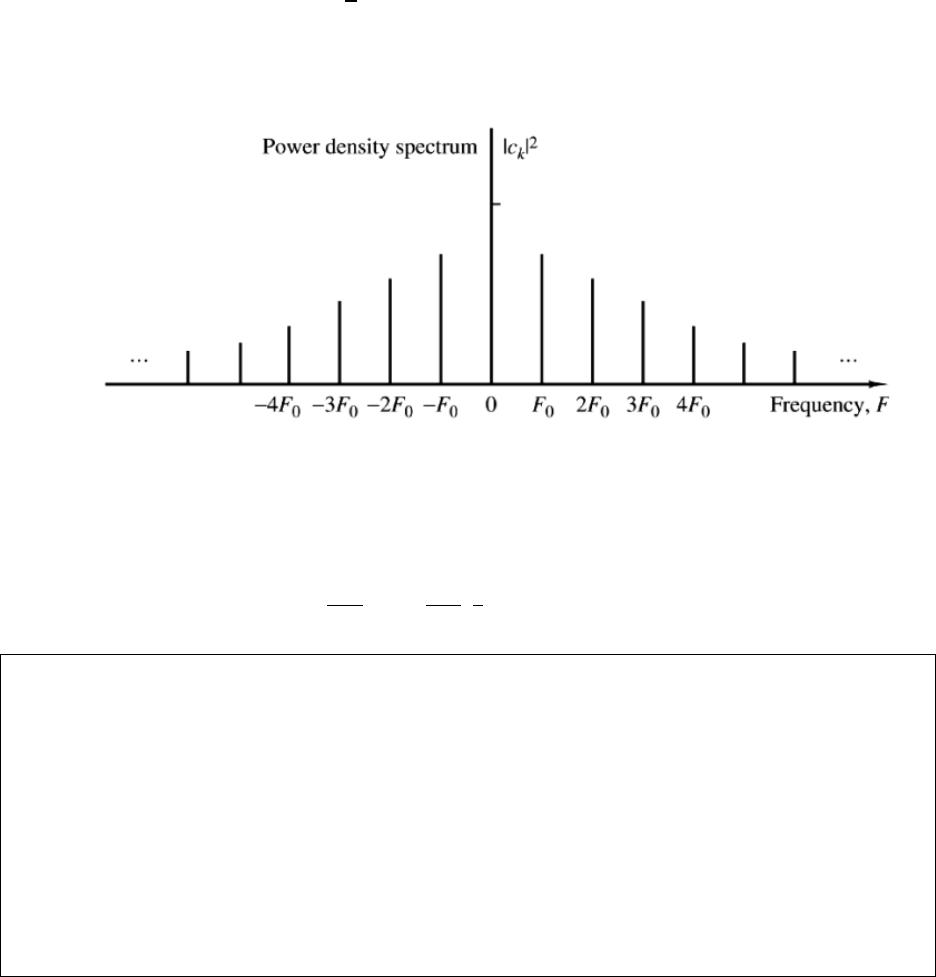
Power density spectrum:

2 Experimental Procedure

2.1 Experiment 1

Are two discrete signals: 𝑒𝑗2𝜋𝑛

6 and 𝑒𝑗4𝜋𝑛

6+𝜋

4 orthogonal?

%%% Problem 1

clear all;

close all;

clc;

syms n;

N=6; %x and yc have period of N=6 (2pi*n/6 and j*4*pi*n/6)

x=exp((j*4*pi*n/6)+pi/4);

yc=exp(-j*2*pi*n/6);

f=simplify(x*yc);

V = subs(f, n, 0:N);

International University School of Electrical Engineering

S_sum = sum(V);

fprintf(‘Inner product is: %f

+j*%f\n’,double(real(S_sum)),double(imag(S_sum)))

if (double(real(S_sum))==0&&double(imag(S_sum))==0)

fprintf(‘=>x1 and x2 are orthogonal\n’)

else

fprintf(‘=>x1 and x2 are not orthogonal\n’)

end

2.2 Experiment 2

Check the orthogonality among following time-limited sinusoidal signals:

𝑥1(𝑡)= 𝑒𝑗2𝜋𝑡,𝑥2(𝑡)= 𝑒𝑗2𝜋2𝑡,𝑥3(𝑡)= 𝑒𝑗2𝜋3(𝑡−0.1),𝑥4(𝑡)= 𝑒𝑗2𝜋4(𝑡−0.1),𝑥5(𝑡)= 𝑒𝑗2𝜋3.9𝑡

clc

clear all

%problem2

syms t T

w = 2*pi;

T = 2*pi/w;

x1 = exp(j*2*pi*t);

x2 = exp(j*2*pi*2*t);

x3 = exp(j*2*pi*3*(t-0.1));

x4 = exp(j*2*pi*4*(t-0.1));