Lecture Notes
Quantitative Methods
SLRM 501 (Semester –I)
SESSION 1–10

SCALES OF MEASUREMENT
What do we mean by Measurement?
The process of assigning numbers or labels to different objects under study to represent them
quantitatively or qualitatively is called measurement. It can be understood as means to denote
the amount of a particular attribute that a particular object possesses. There are certain rules
defining the process of measurement; for ex. Number 1 might be assigned to people who are
from South India and Number 2 might be assigned to people who are from North India.
Measurement is done for the attributes of the units under study but not the units themselves. e.g.
The height, weight, age or other such attributes of a person are measured.
This represents a limited use of the term measurement. In statistics, the term measurement is
used more broadly and is more appropriately termed scales of measurement. Scales of
measurement refer to ways in which variables/numbers are defined and categorized. Each scale
of measurement has certain properties, which in turn determines the appropriateness for use of
certain statistical analyses. The four scales of measurement are nominal, ordinal, interval, and
ratio.
Types of Scales of Measurement
Nominal Scale: Nominal variables (also called categorical variable) can be placed into
categories. They don’t have a numeric value and so cannot be added, subtracted, divided or
multiplied. They also have no order; if they appear to have an order then you probably have
ordinal variables instead. For example: Color of the eyes (Black, Green, Aqua, Hazel, etc.),
Gender (Male/Female), True/False.
Ordinal Scale: The ordinal scale contains things that you can place in order. e.g. hottest to
coldest, lightest to heaviest, richest to poorest. Basically, if you can rank data by 1st, 2nd, 3rd
place (and so on), then you have data that’s on an ordinal scale.
Ordinal scales tell us relative order, but give us no information regarding differences between
the categories. For example, in a race if Ram takes first and Vinod takes second place, we do
not know competition was close by how many seconds.

One more example could be rating surveys in restaurants – When a waiter gets a paper or online
survey with a question: “How satisfied are you with the dining experience?” having 0-10
option, 0 being extremely dissatisfied and 10 being extremely satisfied.
Interval Scale: An interval scale has ordered numbers with meaningful divisions, the
magnitude between the consecutive intervals are equal. Interval scales do not have a true zero
i.e. In Celsius 0 degrees does not mean the absence of heat. For example, temperature on
Fahrenheit/Celsius thermometer i.e. 90° are hotter than 45° and the difference between 10° and
30° are the same as the difference between 60° degrees and 80°.
Measurement of Sea Level is another example of an interval scale. With each of these scales
there is direct, measurable quantity with equality of units. In addition, zero does not represent
the absolute lowest value. Rather, it is point on the scale with numbers both above and below it
(for example, -10 degrees Fahrenheit).
Ratio Scale: The ratio scale of measurement is similar to the interval scale in that it also
represents quantity and has equality of units with one major difference: zero is meaningful (no
numbers exist below the zero). The true zero allows us to know how many times greater one
case is than another. Ratio scales have all of the characteristics of the nominal, ordinal and
interval scales. The simplest example of a ratio scale is the measurement of length. Having zero
length or zero money means that there is no length and no money but zero temperature is not an
absolute zero.
Measures of Central Tendency (Review)
An important objective of any statistical analysis is to calculate a single value that represents the
characteristics/properties of the entire data. This single value representing the entire data is
called the ‘central value’ or ‘average’. This value is the point around which all the other values
of the data cluster. Therefore it is known as measure of location and since this value is located
at a central point nearest to other values of the data it is also known as measure of central
tendency.
In other word, a measure of central tendency is a single value that attempts to describe a set of
data by identifying the central position within that set of data. As such, measures of central
tendency are sometimes called measures of central location. They are also classed as summary
statistics.
Objectives of Averaging
1. To find out the representative number for whole data set. For example, a manager need
not look at ages of every trainee of a fresh batch if the average age is calculated by dividing the
total age of all the trainees by number of trainees. This average is a value that enables the
manager to have a overall idea about the characteristics of the huge volumes of data.
2. To enable comparison. Averages help in drawing conclusions about the characteristics of
different sets of data. For example, a manager can use the average sale of two territories to
compare the performance of sales executives of two territories.
3. To derive inferences about a universe from a sample. Averages help a manager to get
valuable inferences about the whole universe by means of sample data. The average calculated
from a sample data gives a reliable idea about the average of the entire universe.
4. Aids in Decision Making. Averages act as benchmarks or standards for managerial control
and decision-making. A production manager may rely on average employee productivity to set
future production targets for individuals and the organization as a whole. Thus these averages
(average turnover, etc.) act as benchmarks for performance appraisal and decision– making in
future.
Types of Averages
There are two types of averages, mathematical averages and positional averages. Mathematical
average consists of the following
Arithmetic Mean (Simple, Weighted, Combined)
Geometric Mean
Harmonic Mean
Positional averages are
Median
Mode
Arithmetic Mean: The mean or arithmetic mean is the most popular and well-known measure
of central tendency.
Calculating Arithmetic Mean for Ungrouped data
Suppose 𝑥1,𝑥2⋯,𝑥𝑛 are ‘n’ observations of a variable 𝑥, the arithmetic mean, denoted by 𝑥̅ is
calculated as
𝑥̅=𝑠𝑢𝑚 𝑜𝑓 𝑎𝑙𝑙 𝑜𝑏𝑠𝑒𝑟𝑣𝑎𝑡𝑖𝑜𝑛𝑠
𝑛𝑢𝑚𝑏𝑒𝑟 𝑜𝑓 𝑜𝑏𝑠𝑒𝑟𝑣𝑎𝑡𝑖𝑜𝑛𝑠=𝑥1+𝑥2+⋯+𝑥𝑛
𝑛=∑𝑥𝑖
𝑛
𝑖=1
𝑛
where, x̅ is the sample mean
i is the set of natural numbers
∑xi
n
i=1 is the sum of all observations
n is the number of observations
Please note: When the mean is calculated for entire population, it is known a population mean
and is denoted by μ. When the mean is calculated is calculated for a sample, it is called as
sample mean and is denoted by x̅ for variable x.
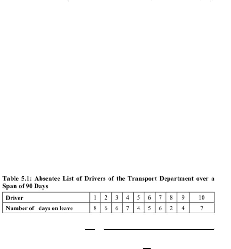
Example: Refer to the data given in the table 5.1. When a manager wants to know the average
number of days a driver is on leave in 90 days, he can calculate the mean of the ungrouped data
as follows:
𝑥̅=∑𝑥
𝑛=8+6+6+7+4+5+6+2+4+7
10
=55
10
=5.5 days per driver
One can calculate the mean using the above method for limited values. But the task becomes
difficult when calculating average for data with large number of observations, say for 5000
employees. In such cases a frequency distribution of the data will be helpful to a manager, and
mean should be calculated using a different method.
Calculating mean from Grouped Frequency distribution
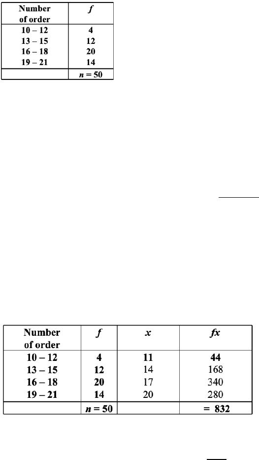
The following table gives the frequency distribution of the number of orders received each day
during the past 50 days at the office of a mail-order company. Calculate the mean.
To compute the arithmetic mean of grouped data, calculate the midpoint of each class and
multiply each midpoint (class mark) by frequency of observations in the corresponding class.
Then add all these results, and divide the sum by the total number of observations.
The formula for calculating Arithmetic mean in grouped frequency data is
x̅=∑fixi
n
i=1
∑fi
n
i=1
where fi is the frequency in each cell
xi is the mid point (class mark) of each class interval
n is the total number of observations
Following table shows the calculations
So, the arithmetic mean will be x̅=832
50 =16.64
Please note that the mean above is referred to as an estimated mean, as we did not use all the 50
observations. The estimate of the value of mean will not be as accurate as the value obtained by
computing from all the 50 observations
Advantages of Arithmetic mean
It is easy to understand and easy to calculate
Every data set has one and only one mean (It is unique)
It takes into account all the observations
It is least affected by fluctuations of sampling
Provides a good basis for comparison
Disadvantages of Arithmetic mean
Mean provides an inaccurate measure in the presence of extreme observations (outliers)
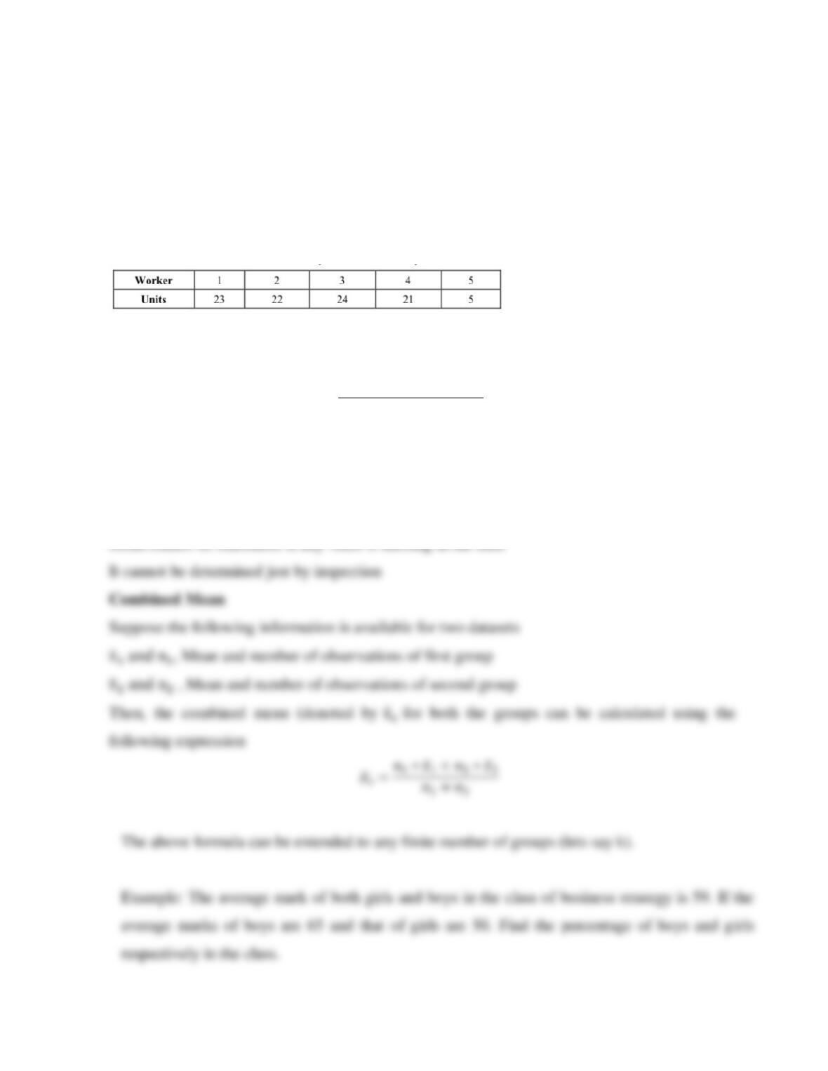
The table above gives the units produced in a day by 5 workers. Then the units produced per
day is
𝑥̅=23+22+24+21+5
5=19 𝑢𝑛𝑖𝑡𝑠
When the mean units are calculated leaving the fifth worker (i.e. 5) the mean is 22.5 units. Thus,
one extreme value ‘5’ has affected the mean. Hence, it is more appropriate to calculate the mean
excluding the extreme value in order to make it more representative.
We cannot calculate the mean for a data set with open-ended classes at either end of the scale.